Chamberlin’s Group Equilibrium: Concept and Theory

In this article we will discuss about Chamberlin’s Group Equilibrium. After reading this article you will learn about: 1. Concept of Industry and Group 2. Theory of Group Equilibrium 3. Assumptions 4. Explanation. 

Concept of Industry and Group:

Group equilibrium relates to the equilibrium of the “industry” under a monopolistic competitive market. The word “industry” refers to all the firms producing a homogeneous product. But under monopolistic competition the product is differentiated.

Therefore, there is no “industry” but only a “group” of firms producing a similar product. Each firm produces a distinct product and is itself an industry. Chamberlin lumps together firms producing very closely related products and calls them product groups.

So in defining an industry, Chamberlin lumps together firms in such product groups as cars, cigarettes, breweries, etc. According to Chamberlin, “Each producer within the group is a monopolist, yet his market is interwoven with those of his competitors, and he is no longer to be isolated from them.”

In the product group, the demand for each product has high cross elasticity so that when the price of other products in the group changes, it shifts the demand curve.

Theory of Group Equilibrium:

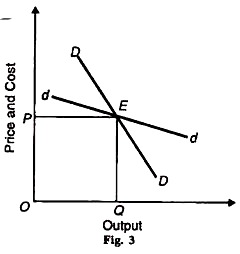
Chamberlin develops his theory of long-run group equilibrium by means of two demand curves DD and dd, as shown in Figure 3. The demand curve facing the group is DD. it is drawn on the assumption that all firms charge the same price and are of equal size, dd represents an individual firm’s demand curve.

The two demand curves reflect the alternatives that face the firm when it changes its price. In the figure, the firm is selling OQ output at OP price. As a member of the group with product differentiation, the firm can increase its sales by reducing its price for two reasons.

First, because it feels that the other firms will not reduce their prices; and second, it will attract some of their customers. On the other hand, if it increases its price above OP, its sales will be re­duced because the other firms in the group will not follow it in increasing their prices and it will also lose some of its customers to the others.

Thus the firm faces the more elastic demand curve dd. But if all firms in the product group reduce (or increase) their prices simultaneously, the firm will face the less elastic demand curve DD.

Assumptions of Chamberlin’s Group Equilibrium:

Prof. Chamberlin’s group equilibrium analysis is based on the following assumptions:

(1) The number of firms is large.

(2) Each firm produces a differentiated product which is a close substitute for the other’s product.

(3) There are a large number of buyers.

(4) Each firm has an independent price policy and faces a fairly elastic demand curve, at the same time expecting its rivals not to take any notice of its actions.

(5) Each firm knows its demand and cost curves.

(6) Factor prices remain constant.

(7) Technology is constant.

(8) Each firm aims at profit maximisation both in the short-run and the long- run.

(9) Any adjustment of price by a single firm produces its effect on the entire group so that the impact felt by any one firm is negligible. This is the symmetry assumption.

(10) As put forth by Chamberlin, there is the “heroic assumption” that both demand and cost curves for all the ‘products’ are uniform throughout the group. This is the uniformity assumption.

(11) It relates to the long-run.

(12) No new firm can enter the group.

Explanation of Chamberlin’s Group Equilibrium:

Given these assumptions and the two types of demand curves DD and dd, Chamberlin explains the group equilibrium of firms. He does not draw the MR curves corresponding to these demand curves and the LMC curve to the LAC curve to simplify the analysis.

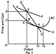
Figure 4 represents the long-run equilibrium of the group under monopolistic competition. Adjustment of long-run equilibrium starts from point A where dd and DD curves intersect each other so that QA is the short-run equilibrium price level at which each firm sells OQ quantities of the product. At this price- output level, each firm earns PABC super-normal profits.

Regarding dd as its own demand curve each firm applies a price cut for the purpose of increasing its sales and profits on the assumption that other firms will not react to its action. But instead of increas­ing its quantity demanded on the dd curve, each firm moves along the DD curve.

In fact, every producer thinks and acts alike so that the dd curve “slides downward” along the DD curve. This downward movement continues until it takes the shape of the d₁d₁ curve and is tangent to the LAC curve at A₁.

This is the long- run group equilibrium position where each firm would be earning only normal profits by selling OQ₁ quantities at Q₁A₁ price. If the d₁d₁ curve slides below the LAC curve, each firm would be incurring losses (not shown in the figure to keep the analysis simple).

Such a situation cannot continue in the long-run and price would have to be raised to the level of A₁ to eliminate losses. Thus each firm will be of the optimum size and operate the optimum scale plant represented by the LAC curve and produce ideal or optimum output OQ₁.