Equilibrium of the Firm and Industry

Equilibrium of the Firm:

Equilibrium indicates a situation in which there is a complete adjustment of the various forces operating there, and there is no inducement to change.

It is an ideal state. That is why a consumer is said to be in equilibrium, when he is deriving maximum satisfaction. Why should he then make any change?

A firm is said to be in equilibrium when it has no incentive either to expand or to contract its output. A firm would not like to change its level of output only when it is earning maximum money profits. Hence, making a maximum profit or incurring a minimum loss is an important condition of a firm’s equilibrium. We shall presently discuss fully the conditions of a firm’s equilibrium.

The equilibrium of the firm is usually discussed in terms of marginal cost and marginal revenue. Now, before explaining the conditions of equili­brium of a firm, it is necessary to describe the concept of marginal revenue and its relation with average revenue.

Average Revenue and Marginal Revenue:

Average revenue must be carefully distinguished from marginal revenue. Average revenue is the revenue per unit of the commodity sold. It is found by dividing total revenue by the number of units sold. But, since different units of a commodity are sold at the same price, in the market, average revenue equals price at which the commodity is sold. Thus, average revenue means price. It is revenue for the seller and price for the consumer.

AR Curve:

It is the same thing as demand curve. Since the consumer’s demand curve is the graphic relation between price and amount demanded, it also represents the average revenue or price at which the various amounts of a commodity are sold, because the price offered by buyers is the revenue from the seller’s point of view. Therefore, average revenue curve of the firm is really the same thing as demand curve of the consumer.

On the other hand, marginal revenue at any level of firm’s output is the net revenue earned by selling another (additional) unit of the product. Algebraically, it is the addition to total revenue earned by selling n units of product instead of no- 1 units, where n is any given number.

The word ‘net’ in the first definition is important. If the price of a product falls when more of it is offered for sale, then that would involve a loss on the previous units, which were sold at a higher price before and will now be sold at the reduced price along with the additional one. This loss in the previous units must be deducted from the revenue earned by the additional unit.

For example, if a firm is selling 7 units of the output at the price of Rs. 16 per unit and if it wants to sell 8 units instead of 7. and thereby the price of the product falls to Rs. 15 per unit, then the marginal revenue will not be equal to Rs. 15 at which the eighth unit is sold, because seven units which were sold at the price of Rs. 16 before will also have to be sold at the reduced price of Rs. 15. That will mean the loss of one rupee on each of the previous 7 units.

The total loss on the previous units would be equal to Rs. 7. Therefore, this loss of 7 rupees should be deducted from the price of Rs. 15 of the eighth unit, while reckoning the marginal revenue. The marginal revenue in this case, therefore, will be Rs. 15 — Rs. 7 = Rs. 8 and not Rs. 15, which is the average revenue.

Marginal revenue can also be directly found by taking out the difference between the total revenue before and after selling the additional unit as follows:

Total revenue when 7 units are sold at the price of Rs. 16 = 7 X 16 = Rs. 112.

Total revenue when 8 units are sold at the price of Rs. 15 = 8 X 15 = Rs. 120.

Therefore, Marginal Revenue or the net revenue earned by the 8th unit= 120— 112= Rs. 8.

Thus, Marginal Revenue of the nth unit

= difference in total revenue in going from n— 1 units to n units.

= Price of nth unit minus loss in revenue on previous units resulting from price reduction.

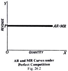
Generally speaking, marginal revenue is less than price as indicated by the above formula. But in perfect competition, when a firm can sell any amount at the ruling market price, marginal revenue is equal to average revenue, since there is no loss incurred on the previous units. Hence, under perfect competition, MR and AR coincide (see Fig. 26.2).

Relationship between Marginal and Average Revenue:

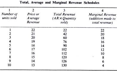
Let us consider the relationship between marginal, average and total revenue at various levels of output more fully with the help of a table given below. This table represents a situation of a hypothetical firm.

Total, Average and Marginal Revenue Schedules:

It is clear from the above table that average revenue and marginal revenue are two different things and, therefore, should not be confused. Column 2 shows the Average Revenue, while Column 4 shows the Marginal Revenue. Marginal Revenue has been derived from the total revenue column of the table. Thus, in going from two to three units, the marginal revenue is 18 and this is found by subtracting 42 from 60, and so forth. The Table further shows that when the average revenue is falling, the marginal revenue is less than the average revenue.

Shape of AR and MR Curves:

Under Imperfect Competition:

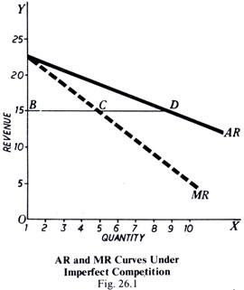
On converting the above schedules of Average Revenue and Marginal Revenue into curves, we get two downward sloping curves and find that marginal revenue curve is below average revenue curve. This is shown in Fig. 26.1. AR is the Average Revenue Curve and MR. the dotted curve, is the Marginal Revenue Curve. This divergence between the average revenue and marginal revenue, as shown in the figure, is actually found when a firm is working under conditions of monopoly or imperfect competition.

It is quite obvious that when price is falling, as indicated by the declining AR curve, the marginal revenue (MR) must always be less than the average revenue (AR), because a falling price must mean some loss on the sale of additional supply. That is why MR curve lies below AR curve.

We have stated above that when average revenue curve falls downward the marginal revenue curve will lie below it (or to the left of it). Now the question arises how far to the left it will lie. When both the marginal revenue curve and the average revenue curve are straight lines and sloping downwards, as shown in the Fig. 26.1, the marginal revenue curve will bisect any line from AR curve drawn perpendicular to the Y-axis. That is, if D is any point on the average revenue curve and if we draw DB a perpendicular from D to the Y-axis, then marginal revenue curve MR must pass through the middle of this perpendicular, i.e., from C where BC = CD.

Under Perfect Competition:

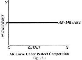
In perfect competition, (Fig. 25.1), the average revenue curve of the firm is a horizontal straight line. This is so because an individual firm under perfect competition by its own action cannot influence the price. The seller, under perfect competition, can sell any amount of the commodity at the ruling market price. In this case when average revenue curve is a horizontal line, marginal revenue curve coincides with the average revenue curve.

This is so because additional units are sold at the same price as before and no loss is caused on the previous units, which would have resulted if the sale of additional units had forced the price down. The average revenue and marginal revenue curves of a firm under perfect competition are shown in Fig. 26.2.

Conditions of Firm’s Equilibrium:

We are now in a position to discuss the conditions of equilibrium of the firm. Here we shall attempt only an analysis of the conditions of firm’s equilibrium in general and not with reference to any particular market form.

Assumptions:

Before explaining firm’s equilibrium, we assume that the entrepreneur, i.e., the owner of the firm, is rational. The rationality on the part of the entrepreneur implies that he tries to maximize his money profits. This is a fundamental assumption in theory of production, and without this the equili­brium of the firm cannot be easily explained. We further assume that the firm produces only one product.

Our conditions would, however, remain valid also in the case of a multi-product firm. But when a firm produces two goods or more, certain other complications arise, which we wish to avoid at this stage. The equilibrium of the firm can be explained with the aid of marginal revenue and marginal cost curves.

There are two conditions of a firm’s equilibrium which we discuss below:

First Condition: Equality of MR and MC:

A firm will be in equilibrium when it is earning maximum profits:

It is obvious that total profits can be increased by expanding output as long as the addition to revenue resulting from the sale of an extra unit of output is greater than the addition to cost caused by producing that extra unit. Now the additions to total revenue and total cost due to an extra unit of output are nothing else but marginal revenue and marginal cost respectively. Thus, a firm will go on expanding output as long as marginal revenue exceeds marginal cost ofproduction.

If at any output, marginal revenue falls short of marginal cost, i.e., an additional unit of output adds less to the revenue than to the cost, the firm will contract output, to avoids a loss and thus increase its profits. The level of output, where marginal revenue and marginal cost are equal, is the point of maximum profit.

Before this point of equality of marginal revenue with marginal cost is reached, the firm will be increasing its total profits by producing more, as it is adding more to the revenue than to the cost’. But if production is carried beyond this point of equality, the profits will start decreasing as the extra revenue will be smaller than the extra cost of production of a unit of output.

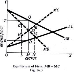
The whole argument can be explained with the help of Fig. 26.3 in which MC is the marginal cost curve and MR the marginal revenue curve. AC and AR are the average cost and average revenue curves respectively. At Output OM, marginal cost equals marginal revenue. This represents the point of maximum profits, and hence of equilibrium.

At outputs smaller than OM, marginal revenue exceeds marginal cost, and hence there is scope for increasing profits by increasing output. For example, at output OL, marginal revenue is LG and marginal cost is LH and LG is greater than LH. It means that by producing the Lth ‘unit, the firm is adding more to revenue than to its cost and, therefore, it will be profitable for it to produce the Lth unit.

Similarly, for every other unit fill the Mth one, the marginal revenue exceeds marginal cost, and, therefore, the firm can increase its total profits by producing up to OM output. If the firm stops producing at OL, the units of output which could have added more money to the firm’s revenue than to its cost would not have been produced and profits would have been smaller by the area GHE than they could have been at output OM. Thus, a. firm has an incentive to produce up to OM level of output.

If the output is increased beyond OM. marginal cost would- exceed -marginal revenue and the production of each additional unit beyond OM output would add more 10 costs than to revenue. For example, at ON output, the marginal cost is KN and marginal revenue is SN, and KN is greater than SN. Thus, production of additional units beyond OM would involve losses and thus reduce total profits. Therefore, the firm would not like to produce beyond OM.

Hence, we conclude that profits are maximum and the firm is in equilibrium when Marginal Cost = Marginal Revenue. This is, however, only one condition, i.e. it is a necessary condition but not a sufficient condition.

In Fig. 26.3, total profits earned by the firm in the equilibrium position can be easily found. At output OM, the average cost is DM, while the average revenue is QM. Hence, the profit per unit will be equal to QD and the total profits will be equal to the rectangle QDRT. Second Condition: MC Cutting MR from Below.

The second condition of a firm’s equilibrium is that the marginal cost curve must cut the marginal revenue curve from below. The condition that for a firm to be in equilibrium marginal cost must equal marginal revenue is no doubt a necessary condition, but not a sufficient condition of equilibrium. For attaining equilibrium, a second condition must also be satisfied.

This is that MC must cut the MR from below at the point of equilibrium. In other words, beyond the equilibrium output, marginal cost must be greater than marginal revenue. If this condition is not met, a firm will not be earning maximum profits, and hence will not be in equilibrium.

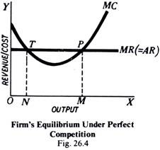
In Fig. 26.4, the point P (i.e., at output OM) satisfies this second condition also, as the MC curve cuts the MR curve from below at P. Beyond the point, P, MC is greater than MR, and it will clearly be not profitable to expand output beyond OM.

There can, however, be cost-revenue situation, which satisfies the first condition of MC being equal to MR, but does not satisfy the second condition of MC cutting MR curve from below. This is shown in Fig. 26.4. In this figure, MR is the straight line marginal revenue curve (as we have already seen, a straight line marginal revenue curve is actually faced by a firm under perfect competition). MC represents the marginal cost of the firm. At point T, the two curves intersect and, therefore, the marginal cost equals marginal revenue. But from the figure it is clear that at T, marginal cost curve.

MC is cutting marginal revenue curve MR from above and, therefore, marginal cost is less than the marginal revenue beyond the point T. Obviously, T cannot be a position of equilibrium since after T marginal cost is less than marginal revenue, and it will be profitable for the firm to expand output. At T or at output ON, the firm instead of making maximum profit is making maximum losses.

At point P, however, in the same figure marginal cost curve is cutting marginal revenue curve from below and marginal cost beyond point P is greater than marginal revenue and, therefore, if the firm expands output beyond P, it will be adding more to cost than to revenue—clearly an unprofitable move. Hence, in Fig. 26.4, point P, and not point T, is the profit-maximizing point. In this equilibrium position, the firm is producing equilibrium output OM.

Thus, we conclude that, for a firm to be in equilibrium position, two conditions must be satisfied under perfect competition:

(i) MC = MR; and

(ii) MC curve must cut MR curve from below at the equilibrium output.

These two conditions of equilibrium hold good in the short run as well as in the long run. Whether the period is short or long, a firm aims at the maximisation of profits, and the profits are maximised only when the above two conditions are satisfied. But one difference remains. In the short run, it is the short-run marginal cost curve, and, in the long run, it is the long-run marginal cost curve which is relevant for comparing with the marginal revenue curve.

Again, these two fundamental conditions, of marginal cost being equal to marginal revenue, and MC curve cutting MR curve from below, are valid whether a firm is working under perfect competition, monopoly or imperfect competition. The difference lies only in the shape of the marginal revenue and marginal cost curves.

Equilibrium of Industry:

Meaning of Equilibrium of Industry:

The concept of equilibrium of industry is of great importance in the analysis of price determination, particularly in product-pricing. An industry is said to be in equilibrium when there is no tendency for its output to increase or decrease. Now the output of the industry can vary, firstly by the expansion or contraction of output by the individual firms, and, secondly, by the entry or exit of the firms. Thus, an industry would he in equilibrium when neither the individual firms have incentive to change their output nor is there any tendency for new firms to enter or the existing firms to leave it.

Conditions of Equilibrium:

The following two conditions must be satisfied if there is to be the equilibrium of the industry:

(a) Each and every firm in the industry should be in equilibrium. This will happen at that output of a firm where marginal cost is equal to marginal revenue and marginal cost curve cuts the marginal revenue curve from below at the equilibrium point.

(b) The second condition is that the industry as a whole should be in equilibrium, i.e., there should be no tendency for the firms either to move into or out of the industry. This will happen when all the entrepreneurs, i.e., owners of the firms of the industry, are earning only ‘normal profits’, that is profits which are just sufficient to induce them to stay in the industry, and when no entrepreneur outside the industry thinks that he could earn at least his normal profits if he were to enter it.

An industry will be earning normal profit if the price (AR) is equal to average cost (AC). If the price is higher, then obviously more than normal profits are being made and new firms will be attracted to the industry. If, on the other hand, price is less than the average cost, the profits are less than the normal and some firms will leave the industry. In both these cases, clearly the industry is not in equilibrium. It will be in equilibrium when AR = AC.

Thus, two conditions are necessary for equilibrium in industry:

(i) MR = MC for all firms and

(ii) AR = AC.

It is rarely that an industry can attain full equilibrium in the short run because although the individual firm in the industry may be in equilibrium in the short run when MR = MC, yet they may be earning supernormal profits, so that there will be inducement for outside firms to enter the industry. Or possibly, the firm may be in equilibrium and may yet be incurring losses, so that some of them would have a tendency to leave the industry.

Hence, in the short run while all firms in the industry may be in equilibrium, the industry is most unlikely to be in equilibrium. Rarely will all the individual firms in the industry are in equilibrium and at the same time make just normal profits, neither more nor less, in the short run. Only in such rare circumstances can the industry attain equilibrium in the short run. This sort of situation is possible only theoretically and has no relevance to the world of reality.

Hence, only in the long run can an industry attain equilibrium, since, in the long run, economic factors can have free and full scope for adjustment. When all the necessary adjustments have taken place, the industry will be in a state of full equilibrium’, i.e., all the individual firms in the industry are in equilibrium and the industry itself is also in equilibrium.