Marris’s Model of the Managerial Enterprise (With Diagrams)

I. Goals of the Firm:

The goal of the firm in Marris’s model is the maximisation of the balanced rate of growth of the firm, that is, the maximisation of the rate of growth of demand for the products of the firm, and of the growth of its capital supply:

Maximise g = g_D = g_c

where g = balanced growth rate

g_D = growth of demand for the products of the firm

g_c = growth of the supply of capital

In pursuing this maximum balanced growth rate the firm has two constraints. Firstly, a constraint set by the available managerial team and its skills. Secondly, a financial constraint, set by the desire of managers to achieve maximum job security. These constraints are analysed in a subsequent section. The rationalisation of this goal is that by jointly maximising the rate of growth of demand and capital the managers achieve maximisation of their own utility as well as of the utility of the owners-shareholders.

It is usually argued by managerial theorists that the division of ownership and manage­ment allows the managers to set goals which do not necessarily coincide with those of owners. The utility function of managers includes variables such as salaries, status, power and job security, while the utility function of owners includes variables such as profits, size of output, size of capital, share of the market and public image. Thus managers want to maximise their own utility

U_M = (salaries, power, status, job security)

while the owners seek the maximisation of their utility

U₀ = f* (profits, capital, output, market share, public esteem).

Marris argues that the difference between the goals of managers and the goals of the owners is not so wide as other managerial theories claim, because most of the variables appearing in both functions are strongly correlated with a single variable the size of the firm (see below). There are various measures (indicators) of size capital, output, revenue, market share, and there is no consensus about which of these measures is the best.

However, Marris limits his model to situations of steady rate of growth over time during which most of the relevant economic magnitudes change simultaneously, so that ‘maximising the long-run growth rate of any indicator can reasonably be assumed equivalent to maximising the long-run rate of most others.’ (Marris, ‘A Model of the Managerial Enterprise’.)

Furthermore, Marris argues that the managers do not maximise the absolute size of the firm (however measured), but the rate of growth (= change of the size) of the firm. The size and the rate of growth are not necessarily equivalent from the point of view of managerial utility. If they were equivalent we would observe a high mobility of managers between firms: the managers would be indifferent in choosing between being employed and promoted within the same growing firm (enjoying higher salaries, power and prestige), and moving from a smaller firm to a larger firm where they would eventually have the same earnings and status.

In the real world the mobility of managers is low. Various studies provide evidence that managers prefer to be promoted within the same growing organisation rather than move to a larger one, where the environment might be hostile to the ‘newcomer’ and where he would have to give considerable time and effort to ‘learn’ the mechanism of the new organisation. Hence managers aim at the maximisation of the rate of growth rather than the absolute size of the firm.

Marris argues that since growth happens to be compatible with the interests of the shareholders in general, the goal of maximisation of the growth rate (however measured) seems a priori plausible. There is no need to distinguish between the rate of growth of demand (which maximises the u of managers) and the rate of growth of capital supply (which maximises the U of owners) since in equilibrium these growth rates are equal.

From Marris’s discussion it follows that the utility function of owners can be written as follows

U_owners = f*(gc)

where g_c = rate of growth of capital.

It is not clear why owners should prefer growth to profits, unless g_c and profits are positively related. At the end of his article Marris argues in fact that g_c and IT are not always positively related. Under certain circumstances g_c and II become competing goals (see p. 364 below). Furthermore from Marris’s discussion of the nature of the variables of the managerial utility function it seems that he implicitly assumes that salaries, status and power of managers are strongly correlated with the growth of demand for the products of the firm: managers will enjoy higher salaries and will have more prestige the faster the rate of growth of demand. Therefore the managerial utility function may be written as follows

U_M = f (g_D, s)

where g_D = rate of growth of demand for the products of the firm

s = a measure of job security.

Marris, following Penrose, argues that there is a constraint to g_D set by the decision-making capacity of the managerial team. Furthermore Marris suggests that’s’ can be measured by a weighted average of three crucial ratios, the liquidity ratio, the leverage- debt ratio and the profit-retention ratio, which reflect the financial policy of the firm.

As a first approximation Marris treats V as an exogenously determined constraint by assuming that there is a saturation level for job security above the saturation level the marginal utility from an increase in V (job security) is zero, while below the saturation level the marginal utility from an increase in ‘s’ is infinite. With this assumption the managerial utility function becomes

U_M = f(g_D)s

where s is the security constraint. Thus in the initial model there are two constraints – the managerial team constraint the job security constraint – reflected in a financial constraint. We will examine these constraints in some detail.

II. Constraints:

The Managerial Constraint:

Marris adopts Penrose’s thesis of the existence of a definite limit on the rate of efficient managerial expansion. At any one time period the capacity of the top management is given there is a ceiling to the growth of the firm set by the capacity of its managerial team. The managerial capacity can be increased by hiring new managers, but there is a definite limit to the rate at which management can expand and remain competent (efficient).

Penrose’s theory is that decision-making and the planning of the operations of the firm are the result of teamwork requiring the co-operation of all managers. Co-ordination and co-operation require experience. A new manager requires time before he is fully ready to join the teamwork necessary for the efficient functioning of the organisation. Thus, although the ‘managerial ceiling’ is receding gradually, the process cannot be speeded up.

Similarly, the ‘research and development’ (R & D) department sets a limit to the rate of growth of the firm. This department is the source of new ideas and new products, which affect the growth of demand for the products of the firm. The work in the R & D department is ‘teamwork’ and as such it cannot be expanded quickly, simply by hiring more personnel for this section: new scientists and designers require time before they can efficiently contribute to the teamwork of the R & D department.

The managerial constraint and the R & D capacity of the firm set limits both to the rate of growth of demand (g_D) and the rate of growth of capital supply (g_c).

The Job Security Constraint:

We said that the managers want job security; they attach (not surprisingly) a definite disutility to the risk of being dismissed. The desire of managers for security is reflected in their preference for service contracts, generous pension schemes, and their dislike for policies which endanger their position by increasing the risk of their dismissal by the owners (that is, the shareholders or the directors they appoint). Marris suggests that job security is attained by adopting a prudent financial policy.

The risk of dismissal of managers arises if their policies lead the firm towards financial failure (bankruptcy) or render the firm attractive to take-over raiders. In the first case the shareholders may decide to replace the old management in the hope that by appointing new management the firm will be run more successfully. In the second case, if the take-over raid is success­ful, the new owners may well decide to replace the old management.

The risk of dismissal is largely avoided by:

(a) Non-involvement with risky invest­ments. The managers choose projects which guarantee a steady performance, rather than risky ventures which may be highly profitable, if successful, but will endanger the managers’ position if they fail. Thus the managers become risk-avoiders.

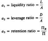
(b) Choosing a ‘prudent financial policy’. The latter consists of determining optimal levels for three crucial financial ratios, the leverage (or debt ratio), the liquidity ratio, and the retention ratio.

The leverage or debt ratio is defined as the ratio of debt to the gross value of total assets of the firm:

The managers do not want excessive borrowing because the firm may become insolvent and be proclaimed bankrupt, due to demands for interest payments and repayment of loans, notwithstanding the good prospects that the firm may have.

The liquidity ratio is defined as the ratio of liquid assets to the total gross assets of the firm:

Liquidity policy is very important. Too low a liquidity ratio increases the risk of in­solvency and bankruptcy. On the other hand, too high a liquidity ratio makes the firm attractive to take-over raids, because the raiders think that they can utilise the excessive liquid assets to promote the operations of their enterprises. Thus the managers have to choose an optimal liquidity ratio neither too high nor dangerously low. In his model, however, Marris assumes without much justification, that the firm operates in the region where there is a positive relation between liquidity and security: an increase in liquidity increases security.

The retention ratio is defined as the ratio of retained profits (net of interest on debt) to total profits:

Retained profits are, according to Marris, the most important source of finance for the growth of capital. However, the firm is not free to retain as much profits as it might wish, because distributed profits must be adequate to satisfy the share­holders and avoid a fall in the price of shares which would render the firm attractive to take-over raiders. If distributed profits are low the existing shareholders may decide to replace the top management. If the low profits lead to a fall in the price of shares, a take­over raid may be successful and the position of managers is thus endangered.

The three financial ratios are combined (subjectively by the managers) into a single parameter a which is called the ‘financial security constraint’. This is exogenously deter­mined, by the risk attitude of the top management. Marris does not explain the process by which a is determined. It is stated that it is not a simple average of the three ratios, but rather a weighted average, the weights depending on the subjective decisions of managers.

Two points should be stressed regarding the overall financial constraint a.

First:

Marris postulates that the overall a is negatively related to a_1, and positively to a₂ and a₃. That is, a increases if either the liquidity is reduced, or the debt ratio is raised by increasing external finance (loans), or the proportion of retained profits is increased. Similarly, a declines if the managers increase the liquidity of the firm, or reduce the pro­portion of external finance (D/A), or reduce the proportion of retained profits (that is, increase the distributed profits), or a combination of all three.

Secondly:

Marris implicitly assumes that there is a negative relation between ‘job security’ (s) and the financial constraint a: if a increases (by either reducing a₁ or in­creasing a₂ or increasing a₃) clearly the position of the firm becomes more vulnerable to bankruptcy and/or to take-over raids, and consequently the job security of managers is reduced. Thus a high value of a implies that the managers are risk-takers, while a low value of a shows that managers are risk-avoiders. The financial security constraint sets a limit to the rate of growth of the capital supply, g_c, in Marris model.

III. The Model: Equilibrium of the Firm:

The managers aim at the maximisation of their own utility, which is a function of the growth of demand for the products of the firm (given the security constraint)

U_managers = f (g_D)

The owners-shareholders aim at the maximisation of their own utility which Marris assumes to be a function of the rate of growth of the capital supply (and not of profits, as the traditional theory postulated)

U_owners = f (g_C)

The firm is in equilibrium when the maximum balanced-growth rate is attained, that is, the condition for equilibrium is

g_D = g_C — g* maximum

The first stage in the solution of the model is to derive the ‘demand’ and ‘supply’ functions, that is, to determine the factors that determine g_D and g_c.

Marris establishes that the factors that determine g_p and g_c can be expressed in terms of two variables, the diversification rate, d, and the average profit margin, m.

The Instrumental Variables:

The firm will first determine (subjectively) its financial policy, that is, the value of the financial constraint a, and subsequently it will choose the rate of diversification d, and the profit margin m, which maximise the balanced-growth rate g*.

The following are policy variables in the Marris model:

Firstly, a implies freedom of choice of the financial policy of the firm. The firm can affect its rate of growth by changing its three security ratios (leverage, liquidity, dividend policies).

Secondly, the firm can choose its diversification rate, d, either by a change in the style of its existing range of products, or by expanding the range of its products.

Thirdly, in Marris’s model price is given by the oligopolistic structure of the industry.

Hence price is not actually a policy variable of the firm. The determination of the price in the market is very briefly mentioned in Marris’s article. He argues that eventually a price structure will develop in which the market shares are stabilized. This equilibrium will be arrived at either by tacit collusion, or after a period of war during which price competition, advertising, product variation or all three weapons are used.

The length of time involved and the level of price and the number of firms which will remain in business is uncertain, due to ‘imperfect knowledge of the competitors’ strength, determination, and skill”, and from the unpredictability of games containing chance moves.

From this line of argument it seems that Marris is not concerned with price determination in oligo­polistic markets, but rather takes it for granted that a price structure will eventually develop. Thus Marris seems to treat price as a parameter (given) rather than as a policy variable at the discretion of the firm. Similarly, Marris assumes that production costs are given.

Fourthly, the firm can choose the level of its advertising. A, and of its research and development activities, R&D. Since the price, P, and the production costs, C, are given, then it is obvious that a higher A and/or R&D expenditures will imply a lower average profit margin and, vice versa, a low level of A and/or R&D implies a higher average profit rate. Implicit in Marris’s model is the average-cost pricing rule

P = C + A + (R & D) + m

where P = price, given from the market

C = production costs, assumed given

A = advertising and other selling expenses

R & D = research and development expenses

M = average profit margin

Clearly m is the residual

M = P – C – (A) – (R & D)

Given p and C, m is negatively correlated with the level of advertising and R & D ex­penditures. Thus m is used as a proxy for the policy variables A and R&D.

In summary, all the policy variables are combined into three instruments:

a, the financial security coefficient

d, the rate of diversification

m, the average profit margin

The next step is to define the variables that determine the rate of growth of demand, g_D, and the rate of growth of supply, g_c, and express these rates in terms of the policy variables, a, d and m.

The rate of growth of the demand: g_D

It is assumed that the firm grows by diversification. Growth by merger or take-over is excluded from this model.

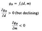
The rate of growth of demand for the products of the firm depends on the diversific­ation rate, d, and the percentage of successful new products, k, that is,

g_D = f₁ (d, k)

where d = the diversification rate, defined as the number of new products introduced per time period, and k — the proportion of successful new products.

Diversification May Take Two Forms:

Firstly, the firm may introduce a completely new product, which has no close substitutes, which creates new demand and thus competes with other products for the income of the consumer. (Marris seems to narrow his analysis to firms producing consumers’ goods.) This Marris calls differentiated diversification, and is considered the most important form in which the firm seeks to grow, since there is no danger of encroaching on the market of competitors and hence provoking retaliation.

Secondly, the firm may introduce a product which is a substitute for similar commodities already produced by existing competitors. This is called imitative diversification, and is almost certain to induce competitors’ reactions. Given the uncertainty regarding the reactions of competitors the firm prefers to diversify with new products. The greater d, the higher the rate of growth of demand.

The proportion of successful new products, k, depends on the rate of diversification d, on their price, the advertising expenses, and the R & D expenditure, as well as on the intrinsic value of the products

k = f₃ (d, P, A, R&D, intrinsic value)

Regarding the intrinsic value of the new product Marris seems to adopt Galbraith’sand Penrose’s thesis (rather far-fetched) that a firm can sell almost anything to the consumers by an appropriately organised selling campaign, even against consumers’ resistance. He implicitly combines intrinsic value with price, that is, price is associated with a given intrinsic value. Price is assumed to have reached equilibrium in some way or another. Thus price is taken as given, despite the fact that the product is new.

k depends on the advertising, A, the R & D expenditures and on d. The higher A and/or R&D, the higher the proportion of successful new products and vice versa. Marris uses m, the average profit margin as a proxy for these two policy variables. Given that m is negatively related to A and R&D, the proportion of successful new products is also negatively correlated with the average profit margin.

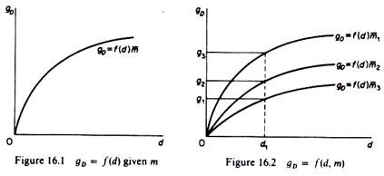
Finally, k depends on d, the rate of new products introduced in each period if too many new products are introduced too fast, the proportion of fails increases. Thus, although the rate of growth of demand, g_D, is positively correlated with the diversific­ation rate (d), g_D increases at a decreasing rate as d increases, due to the rate of intro­duction of new products outrunning the capacity of the personnel involved in the devel­opment and the marketing of the products.

There is an optimal rate of flow of ‘new ideas’ from the R & D department of the firm. If the research team is pressed to speed up the development process of new products there is no time to ‘research’ the product and/or its marketability adequately. Furthermore, top management becomes overworked when the rate of introduction of new products is high, and the proportion of unsuccessful products is bound to increase.

In summary

The g_D function is shown in figures 16.1 and 16.2.

The average rate of profit is constant along any g_D curve. But the curve shifts down­wards as m increases (m₁ < m₂ < m₃). This is due to the negative relationship between g_D and m. With a given rate of diversification (for example, at d₁ in figure 16.2) and given the price of the products, the lower m, the larger the A and/or the R & D expenses, and hence the larger the proportion of successful products and the higher the growth of demand (g₃ > g₂ > g₁). Of course the monotonic positive relationship between d and A (and R & D), which is implied by Galbraith’s and Penrose’s hypothesis and is adopted by Marris, is highly questionable on a priori and empirical grounds.

The Rate of Growth of Capital Supply:

It is assumed that the shareholder-owners aim at the maximisation of the rate of growth of the corporate capital, which is taken as a measure of the size of the firm. Corporate capital is defined as the sum of fixed assets, inventories, short-term assets and cash reserves. It is not stated why the shareholders prefer growth to profits in periods during which growth is not steady.

The rate of growth is financed from internal and external sources. The source of in­ternal finance for growth is profits. External finance may be obtained by the issue of new bonds or from bank loans. The optimal relation between external and internal finance is still strongly disputed in economic literature.

Marris takes the position that the main source of finance for growth is profits, on the following grounds. Firstly, the issue of new shares as a means of obtaining funds is, for prestige and other reasons, not often used by an established firm. Secondly, external finance is limited by the security attitude of managers, that is, from their desire to avoid mass dismissal. Financial security is achieved by setting an upper limit to the debt/assets ratio (leverage) and a lower limit to the liquidity ratio in the long run.

Although profits are the main source of finance for growth, the top management can­not retain as much profits as it would like. There is an upper limit to the ‘retention ratio’, set by the desire of managers to distribute a satisfactory dividend, which will keep shareholders happy and avoid a fall in the prices of shares. Otherwise the selling of shares, or a successful take-over raid, would endanger the position of managers.

The three security ratios are subjectively determined by the managers through the security parameter a, which is a determinant of the retained profits, and hence a deter­minant of the rate of growth of capital.

Under Marris’s assumptions the rate of growth of capital supply is proportional to the level of profits

g_C = a(Π)

where a = the financial security coefficient

Π = level of total profits

The security coefficient a is assumed constant and exogenously determined in this model. This assumption is relaxed at a later stage. It should be stressed, however, that so long as a is constant, growth, g_c, and profits, Π, are not competing goals, but are positively related higher profits imply higher rate of growth.

The next step is to express g_c in terms of the policy variables d and m. The level of total profits depends on the average rate of profit, m, and on the efficiency of the performance of the firm as reflected by its overall capital output ratio, K/X:

Π = f₄ (m, K/X)

It is intuitively obvious that n and m are positively correlated (an increase in the aver­age profit margin results in an increase in the total profits)

∂Π/ ∂m > 0

The relationship between Π and the capital/output ratio is more complicated. The capital/output ratio is claimed to be a measure of efficiency of the activity of the firm, given its human and capital resources. The overall K/X ratio is not a simple arithmetic average of the capital/output ratios of the individual products of the firm, but is a func­tion of the diversification rate d

(K/X) = f₅ (d)

Given K, the relation between X and d is up to a certain level of d positive, reaches a maximum, and subsequently output declines with further increases in the number of new products the overall output increases initially with d due to a better utilization of the team in the R & D department as well as of the skills of the existing managerial team.

Output reaches a maximum when the d is at its optimum level allowing the optimal use of the managerial team and the R & D personnel. Beyond that point, the total output X decreases with further increases in d, and the efficiency of the firm falls the R&D per­sonnel are overworked and the decision-making process becomes inefficient, as there is not enough time allowed for the development of new products or for the study of their marketability. Hence the success rate for new products falls and efficiency declines.

Substituting for K/X in the profit function we obtain

Π = ƒ₄ (m, d)

The relationship between n and d is initially positive, reaches a maximum, and then declines as d is further accelerated.

We next substitute Π in the g_c function

g_C = a.[f₄(m, d)]

The rate of growth of capital is determined by three factors the financial policies of the managers, the average rate of profit and the diversification rate.

Marris assumes in his initial model that a is a constant parameter exogenously deter­mined by the risk-attitude of managers, while there is a positive relation between g_c and m

∂g_C / ∂m > 0

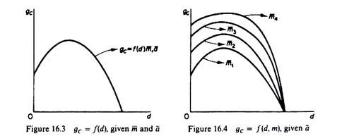
The relationship between g_c and d is not monotonic. The rate of growth of capital, g_c, is positively correlated with d up to the point of optimal use of the R & D personnel and the team of managers; but g_c is negatively correlated with d beyond that point a higher d implies hastening up of the diversification process → inefficient decisions → fall in the overall profit level → low availability of internal finance and consequently a lower rate of growth g_c.

The relation between g_c and d, keeping a and m constant, is shown in figure 16.3. If we allow both d and m to change, while keeping a constant, we obtain a family of g_c = f₂ (d, m) curves (figure 16.4). The average profit rate is depicted as a shift factor of the g c = f(0) curve. The higher the average profit rate, the further from the origin the g_c curves will be (m₁ < m₂ < m₃). These curves are drawn under the assumption that a is constant. (The effects of a change in a are discussed in section IV below.)

Summarising the above arguments, we may present Marris’s model in its complete form as follows:

g_D = f₁(m, d) – (demand-growth equation)

Π = f₄(m, d) – (profit equation)

g_C = a.[f₄(m, d)] – (supply-of-capital equation)

a < a* (security constraint)

g_D = g_c (balanced-growth equilibrium condition)

a is exogenously determined by the risk-attitude of managers. The level of profit Π is endogenously determined. The variables m and d are the policy instruments. Given the balanced-growth equilibrium condition, we have in fact one equation in two unknowns (m and d, given a)

f₁(m, d) = a.[f₄(m, d)]

Equilibrium of the firm:

Clearly the model cannot be solved (is under identified), unless one of the variables m or d is subjectively determined by the managers. Once the managers define a and one of the other two policy variables, the equilibrium rate of growth can be determined.

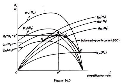
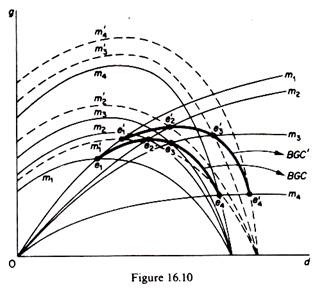
The equilibrium of the firm is presented graphically in figure 16.5, formed by super­imposing figures 16.2 and 16.4. Given their shapes, the g_D and g_c curves associated with a given profit rate intersect at some point. For example, the g_D and g_c curves corres­ponding to m, intersect at point A; the g_D and g_c curves associated with m₂ intersect at point B, and so on. If we join all points of intersection of g_D and g_c curves corresponding to the same level of m we form what Marris calls the balanced-growth curve (BGC), given the financial coefficient a.

The firm is in equilibrium when it reaches the highest point on the balanced-growth curve. The firm decides its financial policy, denoted by a. It next chooses subjectively a value for either m or d. With these decisions taken, the firm can find its maximum bal­anced-growth rate, consistent with a and with the chosen value of one of the other two policy variables. In figure 16.5 the BGC corresponding to a is ABCD.

The balanced- growth rate g* is defined by the highest point B of this BGC. This g* rate is compatible with a unique pair of values of the policy variables, m* and d*. If the firm chooses d*, then m* is simultaneously determined; alternatively, if the firm chooses m*, then d* is simul­taneously determined from the function

g* = ƒ₁ (m*, d*) = a. [ƒ₄ (m*, d*)]

Substituting m* and d* in the profit function

Π = a[ƒ₄ (m, d)]

we find the level of profit, Π*, required to finance the balanced-growth rate, g*. Thus profit is endogenously determined in Marris’s model. Furthermore, growth and profit are not competing goals (so long as a is constant). From the g_c function

g_c = a . (Π)

it is obvious that higher profit implies higher growth rate. However, if the financial coefficient a is allowed to vary, then profits and growth become competing goals.

The question is does the BGC have a maximum? Marris argues that so long as either (or both) of the g_c or g_D curves flattens out or bends, there will always be a maximum point on the BGC curve. Furthermore, depending on the shape of the g_c and the g_D curves, the BGC may be platykurtic, that is, have a flat stretch which indicates that there are several optimal solutions the g* may be achieved by a large number of com­binations of the values of the policy variables m and d (given a is already chosen).

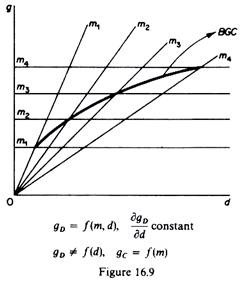
It is only if the g_c curve is parallel to the 4-axis (g_c = ƒ(m) but g_c ≠ ƒ(d)) and the g_D curves are straight upwards-sloping curves (implying that g_D = ƒ(d, m), but k ≠ ƒ(d) and hence the g_D curve does not flatten out) that the BGC increases continuously, never reaching a maximum. This situation is, however, improbable given the capacity for efficient de­cision making of the managerial team and the capacity for well-explored new products of the R & D department of the firm.

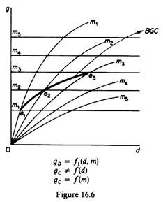
These cases are graphically shown in figures 16.6-16.9. Figure 16.6 depicts the case where g_c ≠ (d), while g_D = f(d, m). The g_c curve becomes parallel to the d-axis, show­ing that g_c does not vary as d increases. The g_c curve shifts upwards (parallel to itself) as the average profit margin increases, given that g_c and m are positively related. The balanced-growth curve has a maximum defined by the curvature of the g_D = f (m, d) function (the maximum g occurs at point e₃ in figure 16.6).

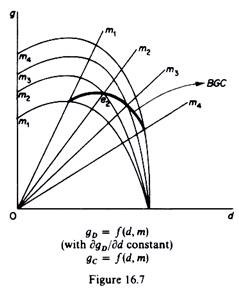
Figure 16.7 depicts the case where g_n = ƒ_x(m, d), and g_c = ƒ₂(d, m). But the curve g_D becomes a straight line through the origin, showing that g_D has a constant slope irrespective of changes in the diversification rate. The g_D curve (line) shifts downwards towards the x-axis as m increases. The balanced-growth curve has still a maximum (e₂) due to the curvature of the g_c function.

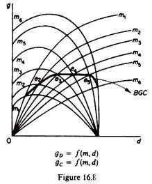
Figure 16.8 shows a platykurtic balanced-growth curve the g_D and g_c functions have several points of intersection (due to their shapes) that lie on a straight line. The flat part of the balanced-growth curve implies that the same optimal (maximum) g* may be achieved by a very large number of combinations of m and d.

Finally figure 16.9 shows the improbable case a balanced-growth curve which never reaches a maximum (explosive growth).

IV. Maximum Rate of Growth and Profits:

Marris argues that in the real world the financial coefficient a is not a constant, but varies. Changes in a clearly affect g_c, given

g_c = a(Π) = a [ƒ₄(m, d)]

A change in a will shift the g_c curves if a increases the g_c curves will shift upwards, while if a is reduced the g_c curves will shift downwards. The new set of g_c intersects the given set of g_D curves at new points, which form a new balanced-growth curve. Given that the relationship between g_c and a is positive (∂g_D/∂a > 0), an increase in a leads to an increase in the rate of growth.

An increase in a will occur if one or more of the three security ratios changes as follows a is higher if the liquidity ratio (a₁) is lowered; or if the debt ratio (a₂) is increased; or if the retention ratio (a₃) is increased. This is due to the fact that a is positively related to a₂ and a₃, but negatively related to a_y.

Clearly an increase in a, however realised, implies a less ‘prudent’, more risky policy of the managers, since a decrease in the liquidity ratio, or an increase in the indebtedness or an increase in the retained profits (which implies a reduction in the paid dividends) reduces the job security of the managers.

Graphically an increase in a is shown by an upwards shift of the BGC (to the position A’B’C’D’ in figure 16.10). Given the g_D curves, the highest point of the new BGC will be above the highest point of the original BGC. This implies that the balanced rate of growth g cannot be maximised unless a assumes its highest optimal value a*. Con­sequently in equilibrium a – a*, that is, the financial constraint takes the form of equality at equilibrium.

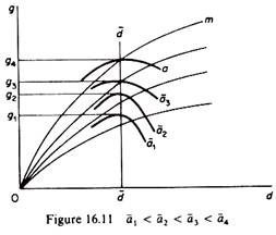
Marris next argues that if a is allowed to vary, growth and profits may become com­peting goals. If a is lowered below its optimum value a* the growth rate is reduced but the profit level, Π, may be raised. A lower value of a (given the d rate) denotes a shift to a lower balanced-growth curve, which implies the intersection of g_D and g_c curves cor­responding to a higher m, and hence a higher n, since n is a positive function of m (figure 16.11).

Thus, although when a is held constant, maximising the growth rate implies maximising profit (g and Π are not competing goals), when a is allowed to vary, growth and profits become competing goals if a is treated as a variable, the firm cannot maxi­mise both the rate of growth and profit.

This explains that under some circumstances managers’ objectives (for higher g) and stockholders’ objectives (for higher Π) may con­flict. It should, however, be clear that a cannot be increased beyond a certain value, determined by the minimum profit requirements of the shareholders; otherwise the job security of managers decreases dangerously.

If the solution of the model does not yield in adequate to satisfy the stockholders, a will be reduced (via, for example, a lowering of the retention ratio), until the maximum obtainable balanced-growth rate is consistent with a level of profit that is satisfactory. This implies that managers seek to maximise the growth rate subject to a minimum profit constraint.

V. Comparison of Marris’s Firm with a Profit Maximiser:

The imposition of either a unit profit tax or a lump tax will lead to a reduction in the level of total profit Π. A growth maximiser will react to a profits tax by reducing his growth rate, reducing his output and raising his price. A profit maximiser will not react to a profits tax in the short run.

An increase in fixed cost will not affect the equilibrium of a profit maximiser in the short run. A growth maximiser, faced with an increase in fixed costs, will react by re­ducing his output and his rate of growth.

The advertising (A) and the research and development (R & D) expenditures will be higher for a growth maximiser than for a profit maximiser.

There will be slack payments to the administrative staff, while slack is zero for a profit maximiser.

The profits of a growth maximiser are smaller than the profits of a profit maximiser.

In the profit-maximisation model Π and q are always positively correlated, while in Marris’s model this positive correlation will be observed only (i) if a is constant and is set equal to its optimal value a*, or (ii) if a* is the same for ail firms in the market (while firms are heterogeneous in respect of efficiency).

If, however, a < a*, or if firms do not have the same a*, then g and n may not be correlated at all, or may even be negatively correlated. Thus, the observed negative correlation coefficient between g and Π, in several applied studies, could be explained by firms having different a*, or setting a < a* (that is, not pursuing a growth-maximising policy).