Measuring Risk: Probability of an Outcome (explained with diagram)

Risk refers to the situation when there is more than one possible outcome of a decision and the probability of each outcome is either known or can be estimated.

Therefore, to measure the degree of risk we need to know the probability of each possible outcome of a decision.

The probability means the likelihood of occurring of an event.

Thus, if possibility of an outcome occurring is 1/4 or 0.25, this means that there is 1 chance in 4 or 25 per cent chance for the outcome to occur. For example, suppose a person is considering to invest in a company which is engaged in the new exploration of offshore oil. If the exploration is successful, the price of company’s stock will rise to Rs. 50 per share and if its exploration meets with a failure, the company’s stock will fall to Rs. 10 per share.

Given these two possible outcomes, namely, Rs. 50 per share price and Rs. 10 per share price, if the past information reveals that the chance of oil exploration being successful is 1/4 or 25 per cent and chance of its failure is 3/4, then we say the probability of success of oil exploration is 25 per cent and the probability of its failure is 75 per cent (The success and failure are the two possible outcomes). Thus probability is a number that indicates the likelihood of an event or outcome occurring.

These are two concepts of probability depending on how it is measured. The first is the frequency concept of probability. If past information or data is available regarding occurrence of outcomes or events, the probability is defined as the proportion of times an outcome occurs if the situation is repeated in the long run over and over again. In general, if a situation is repeated over a large number of times, say M, and if an outcome, say X, occurs m times, then

P (X) m/M

Thus, in our example if we know from the past data of oil exploration that rate of success is 25 per cent, then the probability of getting success is 1/4 or 0.25. The measurement of probability based on the past experience is generally known as the objective measure of probability.

But in many cases there are no similar past situations which help us in measuring probability. In that case the concept of subjective probability is used. The subjective probability is an individual’s personal view about the chance of an outcome to occur and is based on his personal judgement, experience or knowledge about the subject and not on the frequency with which outcome actually took place in the past.

Obviously, when probability is subjectively determined and not based on the past data, the different individuals will attach different probabilities to the occurrence of various outcomes and therefore they will make different choices.

In whatever way the probability is arrived at, it helps us to measure two important concepts, namely, expected value and variability of outcome. With the use of these two concepts we compare the profitability of various strategies involving risk and uncertainty which helps us to make a choice among them. We explain below the meaning of these two concepts.

Measuring Risk with Probability Distribution:

As explained above, the probability of an outcome is the likelihood that an event will occur. Probability distribution describes the occurrence of all possible outcomes of an event and the probability of occurrence of each outcome. It is worth noting that the sum of probabilities of all possible outcomes must equal unity because probabilities of all outcomes together must equal certainty.

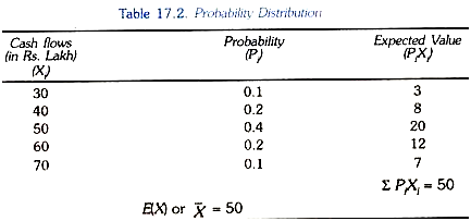
Thus, in Table 17.2 we give all possible cash flows that will occur from an investment project A in the next year and the probabilities of their occurrence. It will be seen from Table 17.2 that there are five possible cash flows in the next year depending on the state of the economy which is determined by general economic conditions, nature of competition in the industry to which the firm belongs. If all conditions are favourable for the firm, its cash flow will be 70 lakhs whose probability is 0.1 or 10 per cent.

On the other hand, if all conditions are unfavourable for the firm, its cash flow from the investment project will be Rs. 30 lakhs whose probability of occurrence is also 0.1 or 10 per cent. One of the other three cash flows will occur if some factors work in favour of the firm’s project A and others unfavourable to it.

The probability distribution shows that there is 10 per cent probability that all determining conditions work in favour of the investment project which yields cash flow of Rs. 70 lakhs in the next year. Similarly, there is 10 per cent probability that all conditions will be unfavourable and yields cash flow of Rs. 30 lakhs in the next year. It is more probable that some conditions will be favourable and others unfavourable for firm’s project so that intermediate cash flows such as Rs. 40 lakhs, 50 lakhs and Rs. 60 lakhs would occur.

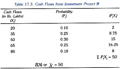
In Table 17.3 we give the cash flows that will occur in the next year and their associated probabilities from an investment project B. It will be seen that cash flows from investment project B are more dispersed as compared to the cash flows from investment project A.

The concept of probability distribution is required for evaluating and comparing investment projects when managers have to take decisions under conditions of risk. From the probability distribution of outcomes we can calculate two values which are essential for decision making under conditions of risk. (1) Expected value of all possible outcomes (cash-flows in our above example), and (2) a value that measures the degree of risk involved.We explain below both of these.

Expected Value:

As stated above, individuals and firms face situations where a number of outcomes can occur each of which results in a certain payoff or cash flow, that is, monetary gain or loss. If the probability of each outcome is known we can find out the expected monetary value in this uncertain situation (that is, when a variety of outcomes can occur). The expected monetary value is the weighted average of payoffs of all possible outcomes with the probability of each outcome used as weights.

Thus the expected value of an uncertain income is the average payoff of the various outcomes. For example, it investment in offshore oil exploration, there are two possible outcomes, namely, the success of the project yielding a payoff of Rs. 50 per share with a probability of 0.25 and the failure yielding a payoff Rs. 10 per share with a probability of 0.75.

Thus in this case, expected value of investment per share:

= 0.25 X 50 + 0.75 x 10

= 12.5 + 7.5

= Rs. 20

In general terms if there are two possible outcomes with payoffs of X₁ and X₂ and the probability of each possible outcome is denoted by P₁ and P₂, then the expected value of investment is given by

Similarly, if there are n possible outcomes, then the expected value is

or in condense form, expected value in case of n possible outcomes with their associated probabilities can be written as

In the data given in Table 17.2 regarding 5 possible cash flows from an investment project, the expected value is obtained by multiplying the possible cash flows with their associated probabilities and then adding them. This we have done in the last column of Table 17.2 whose sum yields 50. Thus

E(X) or x= (0.1 X 30) + (0.2 x 40) + (0.4 x 50) + (0.2 x 60) + (0.1 x 70)

= 3 + 8 + 20+12+ 7 = 50

Risk and Probability Distribution:

In addition to the expected value, the probability distribution of outcomes also helps us in measuring risk involved in a project. In fact, the variability of outcomes measures the degree of risk involved in any choice of a project or strategy from the various alternative projects or strategies. In economics and finance, risk is the measured by the extent of dispersion {i.e. deviation) of possible outcomes from the expected value.

The greater the variability or dispersion of payoff of various outcomes from the expected value of payoff means the greater risk involved. The variability of outcomes may be measured by the average deviation of actual values of payoffs of various outcomes from the expected value of payoff with probability of each being used as weights. Let X₁ and X₂ are the payoffs of two outcomes and the probability of each is P₁ and P₂, then the average deviation (V) as a measure of risk is given by

V = P₁[X₁ – E(X₁)] + P₂ [X₂ – E(X2)]

However, the most widely used measure of dispersion or variability is the standard deviation. The standard deviation (d or σ) is defined as the square root of the weighted average of the squared deviation of all possible outcomes from the expected value with probabilities of various possible outcomes used as weights. Thus, in case of three possible outcomes

Where α is standard deviation and X₁, X₂, X₃ are outcomes and E(X) is the expected value of outcomes.

In general terms, when there are n outcomes, standard deviation (σ) of outcomes is given by,