Utility Theory and Attitude toward Risk (Explained With Diagram)

The underlying principles of making a choice in risky and uncertain situation, namely, expected return and the degree of risk involved apply equally well to other choices.

In this section we focus on examining individual’s choices in the face of risk.

In the various earlier theories of consumer’s behaviour we saw that in making choices among commodity bundles when there is no risk and uncertainty, the consumer maximises his utility. We will analyse below how an individual maximises his expected utility when risk or uncertainty is present.

“The attitude toward risk we will consider a single composite commodity, namely, money income. An individual’s money income represents the market basket of goods that he can buy. It is assumed that the individual knows the probabilities of making or gaining money income in different situations. But the outcomes or payoffs are measured in terms of utility rather than rupees”.

People’s preferences toward risk greatly differ. Most individuals generally prefer the less risky situation (that is, the situation with less variability in outcomes or rewards). In other words, most individuals seek to minimise risk and are called risk averter or risk averse.

However, some individuals prefer risk and are therefore called risk-seekers or risk lovers. Some other individuals are indifferent toward risk and are called risk-neutral. But it is important to note that these different preferences toward risk depend on whether for an individual marginal utility of money diminishes or increases or remains constant.

As shall be explained below, for a risk averse individual marginal utility of money diminishes as he has more money, while for a risk-seeker marginal utility of money increases as money with him increases. In case of risk-neutral individual marginal utility of money remains constant as he has more money.

Risk Averter:

To explain the attitude toward risk we will consider a single composite commodity, namely, money income. An individual’s money income represents the market basket of goods that he can buy. It is assumed that the individual knows the probabilities of making or gaining money income in different situations. But the outcomes or payoffs are measured in terms of utility rather than rupees.

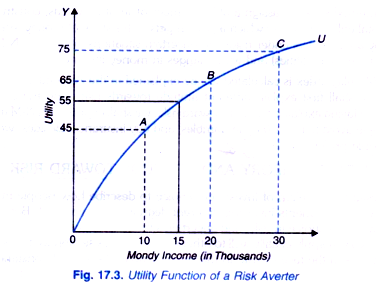
In Fig. 17.3 we have drawn a curve OU showing utility function of money income of an individual who is risk-averse. It will be seen from this figure that the slope of total utility function OL; decreases as the money income of the individual increases. Note that we measure money income on the X-axis and utility on the Y-axis.

It will be seen from Fig. 17.3 that as money income of the individual increases from 10 to 20 thousand rupees, his total utility increases from 45 units to 65 (that is, by 20 units) and when his money increases from 20 thousand to 30 thousand rupees, his total utility increases from 65 to 75 units (that is, by 10 units).

Thus in this concave utility function depicted in Fig. 17.3 marginal utility of money of an individual decreases as his money income decreases and therefore it represents the case of risk-averse individual. Suppose the individual is currently employed on a fixed monthly salary basis of Rs. 15000.

There is no uncertainty about the income from this present job on a the fixed salary basis and hence no risk. Now, suppose that the individual is considering to join a new job of a salesman on a commission basis. This new job involves risk because his income in this case is not certain.

This is because if he proves to be a successful salesman his income may increase to Rs. 30 thousand per month but if he does not happen to be a good salesman his income may go down to Rs. 10 thousand per month. Suppose in this new job there is 50-50, chance of either earning Rs. 30 thousands or Rs. 10 thousands (that is, each has a probability of 0.5). When there is uncertainty, the individual does not know the actual utility from taking a particular action.

But given the probabilities of alternative outcomes, we can calculate the expected utility. Whether the individual will choose the new risky job or retain the present salaried job with a certain income can be known by comparing the expected utility from the new risky job with the utility of the current job. It will be seen from the utility function curve OU in Fig. 17.3 that the utility of money income of Rs. 15,000 with certainty is 55.

Further, in case of new risky job if he is proved to be a successful salesman and his income increases to Rs. 30 thousands, his utility from Rs. 30 thousands is 75, and if he fails as a good salesman, his income falls to Rs 10 thousands which yields him utility of Rs. 45. (Note that in the new risky job, the expected income is 20,000 which is given by E(X) = 0.5 x 10,000 + 0.5 x 30,000 = Rs. 20,000). Given that the probability of success or failure as a salesman is 0.5, the expected utility of the new job is given by,

E (U) = 0.5 U (10,000) + 0.5 U (30,000)

= 0.5 x 45 + 0.5 x 75

= 22.5 + 37.5

= 60.0

Thus with the present job with a fixed salary of Rs. 15,000 with no uncertainty is 55 whereas the expected utility of the new job or salesman on commission basis is 60. Though the individuals is risk-averse as revealed by the nature of his utility function of money income, but since the expected utility of the risky job is greater than the utility of the present job with a certain income he will choose the risky job.

Let us now slightly change the data. Suppose that if the individual in his new job proves to be successful and earns Rs. 30,000, double the present assured income of Rs. 15,000 but if he fails in his new risky job of a salesman on commission basis, his income falls to zero, then the expected utility of the risky job is given by,

E (U) = 0.5 U (0) + 0.5 U (30,000)

= 0 + 0.5 x 75

= 37.5

Now the expected utility from the new risky job is less than the utility of 55 from the present job with an assured income of Rs. 15,000 (Note that in the risky job also, expected income is Rs. 15,000 [E(x) = 0.5 x 0 + 0.5 x 30,000 = 15000], Note again that Figure 17.3 we are considering the choice of a risk averse individual for whom marginal utility of money declines as he has more of it.

We are now in a position to provide a precise definition of risk-averse individual. Precisely speaking, a person who prefers a certain given income to a risky job with the same expected income is called risk averter or risk-averse. Risk aversion is the most common attitude toward risk.

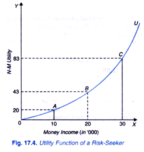
Risk Lover On the other hand, a person is risk-preferred or risk-loving who prefers a risky outcome with the same expected income as a certain income. In case of a risk-loving individual, marginal utility of income to the individual increases as his money income increases as shown by the convex total utility function curve OU in Fig. 17.4.

Suppose this risk-loving individual has a present job with a certain income of Rs. 20 thousands. It will be seen from Fig. 17.4 that the utility of Rs. 20 thousands is 43 units to this individual. Now, if he is offered a risky job with his income of Rs. 30 thousands if he happens to be highly efficient and Rs. 10 thousands if he happens to be not so efficient in the new job with the equal probability of 0.5 in these two jobs, then the expected utility from the new job is given by

E (U) = 0.5 U(10,000) + 0.5 U (30,000)

It will be seen from Fig. 17.4 that the utility of Rs. 10 thousands to this individual is Rs. 20 while utility of Rs. 30 thousands to him is 83. Therefore,

E (U) = 0.5 (20) + 0.5 (83)

= 10 + 41.5

= 51.5

Since the expected utility from the new risky job is 51.5 which is greater than the utility of 43 from the present job with a certain income of Rs. 20 thousands, the risk-loving individual will prefer the new risky job even though the expected income in the new risky job is also Rs. 20,000 as (0.5 x 10,000) + 0.5 (30,000) = Rs. 20,000).

As mentioned above, most of the individuals are risk averse but there is a good deal of evidence of people who are risk seekers. It is risk-loving individuals who indulge in gambling, buy lotteries, engage in criminal activities such as robberies, big frauds even at risk of getting heavy punishment if caught.

Risk-Neutral:

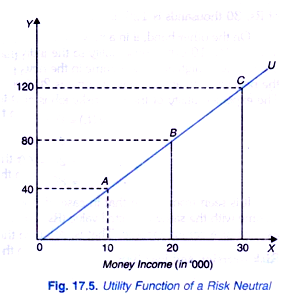
A person is called risk neutral, if he is indifferent between a certain given income and an uncertain income with the same expected value. An individual will be risk neutral if his marginal utility of money income remains constant with the increase in his money. The total utility function of a risk neutral person is shown in Fig. 17.5. It will be seen from this figure that utility of a certain income of Rs. 20 thousands is 80. Now, in a risky job when income increases to Rs. 30 thousands if he proves to be a successful salesman, the utility of Rs. 30 thousands is 120 units.

On the other hand, if in a new risky job, he proves to be a bad salesman, his income goes down to Rs. 10,000 whose utility to the individual is 40 units. We assume that there is equal probability of high and low income in the new risky job. Note that expected value of income in the new job with an uncertain income is 20,000 as (0.5 x 10,000 + 0.5 (30,000) = 20,000. The expected utility of the new risky job is given by

E (U) = 0.5 U (10,000) + 0.5 U (30,000).

= 0.5 (40) + 0.5 (120)

= 20 + 60

= 80

It is seen from above that in case of risk-neutral person expected utility of an uncertain income with the same expected value (Rs. 20,000 in the present case), is equal to utility of an assured or a certain income. That is, risk-neutral person is indifferent between them.

Risk Aversion and Fair Bets:

People differ greatly in their attitudes towards risk. In Bernoulli’s hypothesis we have seen that a person whose marginal utility of money declines will refuse to accept a fair gamble. A fair game or gamble is one in which the expected value of income from a gamble is equal to the same amount of income with certainty. The person who refuses a fair bet is said to be risk averse.

Thus, the risk averter is one who prefers a given income with certainty to a risky gamble with the same expected value of income. Risk aversion is the most common attitude towards risk. It is because of the attitude of risk aversion that many people insure against various kinds of risk such as burning down of a house, sudden illness of a severe nature, car accidence and also prefer jobs or occupations with stable income to jobs and occupations with uncertain income.

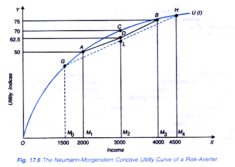
This attitude of risk aversion can be explained with Neumann-Morgenstern method of measuring expected utility. It may be noted that marginal utility of income of a risk-averter diminishes as his income increases. In Figure 17.6 Neumann-Morgenstern utility function curve U (I) has been drawn. It will be seen from this figure that N- M utility curve starts from the origin and has a positive slope throughout indicating that the individual prefers more income to less.

Further the N-M utility curve shown in Figure 17.6 is concave which shows the marginal utility of income of a person diminishes as his income increases. Therefore, the utility curve in Figure 17.6 represents the case of a risk averter or the attitude of risk aversion. With Rs. 2,000 income, the person’s utility is 50 which rises to 70 when his income increases to Rs. 3,000. As his income further increases to Rs. 4,000, his utility rises to 75.

 

Now suppose the person’s current income is Rs. 3,000 and he is offered a fair gamble in which he has a 50-50 chance of winning or losing Rs. 1,000. Thus, the probability of his winning is 1/2 or 0.5. If he wins the game, his income will rise to Rs. 4,000 and if he loses the gamble, his income will fall to Rs. 2,000.

The expected money value of his income in this situation of uncertain outcome is given by:

E (V) = 1/2 x 4000 + 1/2 x 2000 = Rs. 3000

If he rejects the gamble he will have the present income (i.e., Rs. 3,000) with certainty. Though the expected value of his uncertain income prospect is equal to his income with certainty a risk averter will not accept the gamble.

This is because as he acts on the basis of expected utility of his income in the uncertain situation (that is, Rs. 4,000 if he wins and Rs. 2,000 if he loses) can be obtained as under:

Expected Utility (EU) = π U (Rs. 4000) + 1 – π U (Rs. 2000)

As will be seen from Figure 17.6 the utility of the person from Rs. 4,000 is 75 (point B on the utility curve and utility from 2000 is 50 (point A in Figure 17.6), the expected utility from this uncertain prospect will be:

E (U) = 1/2 (75) + 1/2 (50)

= 37.5 + 25 = 62.5

In the N-M utility curve U (I) in Figure 17.6 the expected utility can be found by joining point A (corresponding to Rs. 2,000) and point B (corresponding to Rs. 4,000) by a straight line segment AB and then reading a point on it corresponding to the expected value of the gamble Rs. 3,000, the expected value of the utility is M₂D (= 62.5) which is less than M₂C or Rs. 70 which is the utility of income of Rs. 3,000 with certainty.

Therefore, the person will refuse to accept the gamble (that is, he will not gamble). It should be carefully noted that his rejection of gamble is due to diminishing marginal utility of money income for him. The gain in utility from Rs. 1,000 in case he wins is less than the loss in utility from Rs. 1000 if he loses the gamble. That is why his expected utility from the uncertain income prospect has been found to be lower than the utility he obtains from the same income with certainty.

It follows from above that in case marginal utility of money income diminishes a person will avoid fair gambles. Such a person is called risk averter as he prefers an income with certainty (i.e., whose variability or risk is zero) to the gamble with the same expected value (where variability or risk is greater than zero). Let us illustrate it with another example. Suppose to our person with a certain income of Rs. 3,000, two fair gambles are offered to him. First, a 50:50 chance of winning or losing Rs. 1000 as before and the second a 50:50 chance of winning or losing Rs. 1,500.

With the even chance of winning and losing the expected value of income in the second gamble will be 1/2(1500) + 1/2 (4500) = Rs. 3000. On the N- M utility curve U (I) in Figure 17.6 we draw a straight line segment GH joining point G (corresponding to income of Rs. 1500) and H corresponding to income of Rs. 4500). It will be seen from this straight-line segment GH that the expected utility from the expected money value of Rs. 3,000 from the second gamble is M₂L which is less than M₂D of the first gamble.

Thus the person will prefer the first gamble which has lower variability to the second gamble which has a higher degree of variability of outcome. It should be remembered that risk in this connection is measured by the degree of variability of outcome. In the first gamble, the degree of variability of outcome is less and therefore the risk is less and in the second gamble, the degree of variability is greater which makes it more risky. And in case of income with certainty there is no variability of outcome and therefore involves no risk at all. A risk-averse person therefore prefers the income with certainty to any gamble with the same expected money value as the income with certainty.