Samuelson’s Model of Business Cycle (With Diagrams)

Explanation to the Samuelson’s Model of Business Cycle:

Samuelson in his seminal paper convincingly showed that it is the interaction between the multiplier and accelerator that gives rise to cyclical fluctuations in economic activity.

The multiplier alone cannot adequately explain the cyclical and cumulative nature of the economic fluctuations.

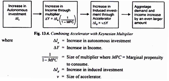
An autonomous increase in the level of investment raises income by a magnified amount depending upon the value of the multiplier. This increase in income further induces the increases in investment through the acceleration effect. The increase in income brings about increase in aggregate demand for goods and services. To produce more goods we require more capital goods for which extra investment is undertaken.

Thus the relationship between investment and income is one of mutual interaction; investment affects income which in turn affects investment demand and in this process income and employment fluctuate in a cyclical manner. We have shown below in Fig. 13.4 how income and output will increase by even larger amount when accelerator is combined with the Keynesian multiplier.

Fluctuations in investment are the main cause of instability in a free private enterprise economy. This instability further increases due to the interaction of the multiplier and accelerator. The changes in any component of aggregate demand produce a multiplier effect whose magnitude depends upon the marginal propensity to consume.

When consumption, income and output increase under the influence of multiplier effect, they induce further changes in investment and the extent of this induced investment in capital goods industries depends on the capital-output ratio, that is, the interaction between the multiplier and accelerator without any external shocks can give rise to the business cycles whose pattern differs depending upon the magnitudes of the marginal propensity to consume and capital-output ratio.

The model of interaction between multiplier and accelerator can be mathematically represented as under:

where Y_t, C_t, it stand for income, consumption and investment respectively for a period t, C_a stands for autonomous consumption, I_a for autonomous investment, c for marginal propensity to consume and v for the capital-output ratio or accelerator.

From the above equations it is evident that consumption in a period t is a function of income of the previous period Y_t-1. That is, one period lag has been assumed for income to determine the consumption of a period. As regards induced investment in period t, it is taken to be the function of the change in income in the previous period. This means that there is two periods gap for changes in income to determine induced investment.

In the equation (iii) above, induced investment equals v(Y_t-1– Y_t-2) or v(∆Y_t-1). Substituting equations (ii) and (iii) in equation (i) we have the following income equation which states how changes in income are dependent on the values of marginal propensity to consume (c) and capital-output ratio v(i.e., accelerator).

This is due to the fact that in static equilibrium, given the data of the determining factors, the equilibrium level of income remains unchanged, that is, in this case, Y_t = Y_t-1 = Y_t-2 = Y_t-n so that period lags have no influence at all and accelerator is reduced to zero. Thus, in a dynamic state when autonomous investment changes, the equation (iv) describes the path which a disequilibrium system follows to reach either a final equilibrium state or moves away from it. But whether the economy moves towards a new equilibrium or deviates away from it depends on the values of marginal propensity to consume (c) and capital-output ratio v (i.e., accelerator).

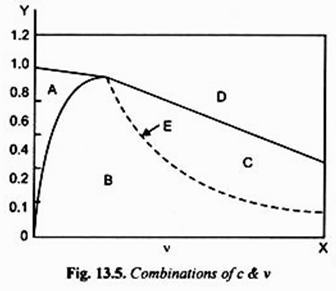
By taking different combinations of the values of marginal propensity to consume (c) and capital- output ratio (v), Samuelson has described different paths which the economy will follow. The various combinations of the values of marginal propensity to consume and capital-output ratio (which respectively determine the magnitudes of multiplier and accelerator) are shown in Fig. 13.5.

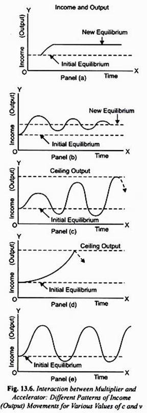
The five paths or patterns of movements which the economic activity (as measured by gross national product or income) can have depending upon various combinations of the values of marginal propensity to consume (c) and capital-output ratio (v) are depicted in Fig. 13.6. When the combinations of the value of marginal propensity to consume (c) and capital-output ratio (v) lie within the region marked A, with a change in autonomous investment, the gross national product or income moves upward or downward at a decreasing rate and finally reaches a new equilibrium as is shown in panel (a) of Fig. 13.6.

If the values of c and v are such that they lie within the region B, the change in autonomous investment or autonomous consumption will generate fluctuations in income which follow the pattern of a series of damped cycles whose amplitudes go on declining until the cycles disappear as is shown in panel (b) of Fig. 13.6.

The region C in Fig. 13.5 represents the combinations of c and v which are relatively high as compared to the region B and determine such values of multiplier and accelerator that bring about explosive cycles, that is, the fluctuations of income with successively greater and greater amplitude.

The situation is depicted in panel (c) of Fig. 13.6 which shows that the system tends to explode and diverges greatly from the equilibrium level. The region D in Fig. 13.5 provides the combinations of c and v which cause income to move upward or downward at an increasing rate which has somehow to be restrained if the cyclical movements are to occur.

This is depicted in panel (d) of Fig. 13.6. Like the values of multiplier and accelerator of region C, their values in region D cause the system to explode and diverge from the equilibrium state by an increasing amount.

In a special case when values of c and v (and therefore the magnitudes of multiplier and accelerator) lie in region E of Fig. 13.5 they produce fluctuations in income of constant amplitude as is shown in panel (e) of Fig. 13.6.

It follows from above that region A and B are alike, they after a disturbance caused by a change in autonomous investment or consumption finally bring about stable equilibrium in the system. On the other hand, the values of c and v and therefore the magnitudes of multiplier and accelerator of region C and D resemble each other but are such that they cause great instability in the system as both of these values cause successively greater divergence from the equilibrium level and the system tends to explode.

The case of region E lies in between the two as the combinations of values of c and v in it are such that cause cyclical movements of income which neither move toward nor away from the equilibrium. It is worth noting that all the above five cases do not give rise to cyclical fluctuations or business cycles.

It is only combinations of c and v lying in regions B, C and E that produce business cycles. The values of accelerator and multiplier in the region A are such that with a disturbance caused by a change in autonomous investment or autonomous consumption, the economic activity (as measured by the level of income or Gross National Product) moves smoothly from an initial equilibrium to a new equilibrium with no cyclical fluctuations or oscillations.

On the other hand, the values of c and v (and therefore of multiplier and accelerator) of the region B produce cyclical fluctuations which are of the type of damped oscillations that tend to disappear over time, that is, the amplitude of the cycles shrinks to zero over a period of time. However, this contradicts the historical experience which reveals that there is no tendency for the cyclical movements to disappear or die out over time.

However, it is worth noting that the case B explains the impact of a single disturbance on income and employment. For example, the effect of a one time increase in autonomous investment goes on diminishing over time if no other disturbance takes place.

However, in reality, further disturbances such as technological advances, innovations, natural disasters and man-made disasters such as security scam in India in 1991-92 do take place quite frequently and at random intervals and in a way they provide shocks to the system.

Thus, the values of c and v of region B can generate cyclical fluctuations over time without dying out if the above-mentioned disturbances are occurring frequently at random. This results in business cycles whose duration and amplitude are quite irregular and not uniform.

As a matter of fact, the business cycles in the real world also reveal such irregular pattern. To sum up, “what otherwise shows up as a tendency for the cycle to disappear in case B may be converted into unending sequence of cycles by the addition of randomly disturbed erratic shock system.”

In case of the values of multiplier and accelerator falling within the region C, though they generate continued oscillations, the cycles produced by them tend to become ‘explosive’ (i.e., their amplitude tends to increase greatly). But they are not consistent with the real world situation where oscillations do not become explosive.

However, the values of multiplier and accelerator falling within region C can be made consistent with the actual world situation by incorporating in the analysis the so called buffers. Buffers are the factors which impose upper limit or ceiling on the expansion of income and output on the one hand or impose a lower limit or floor on the contraction of output and income on the other.

With the inclusion of these buffers the otherwise explosive upward and downward fluctuations arising out of values of multiplier (or MPC) and accelerator (or capital-output ratio) of the region C can become limited cyclical fluctuations, characteristic of the real world situation.

What has been said about case C above also applies to region D where the values of multiplier and accelerator are such that give rise to directly explosive upward or downward movement which can be restrained by the factors determining the ceiling and floor. However, the adequate explanation of the business cycles in this case would require the reasons why the system starts moving in the reverse direction, say, after striking the ceiling.

Hicks in his famous theory of the business cycles provides the reasons which cause movement of the system in the reverse direction after it hits the ceiling or the floor as the case may be. Hicks theory of business cycles will be explained below at length.

Lastly, the case E represents a situation where the business cycles neither try to disappear, nor try to explode, they go on continually with a constant amplitude. This however contradicts the real world situation and is quite impossible. This is because in the real world situation, business cycles differ a good deal in amplitude and duration.

Summing Up:

We have explained the interaction of multiplier and accelerator in case of various values of marginal propensity to consume (c) and capital-output ratio (v). On the basis of the interaction of the multiplier and accelerator the two categories of business cycle theories have been put forward.

One category of these business cycle theories assumes the values of multiplier and accelerator which generate explosive cycles. For example, Hicks’ theory of business cycles falls in this category. On the other hand, Hansen has propounded a business cycle theory based on the interaction of multiplier with a weak accelerator which produces only damped oscillations.

Further, as indicated above, the interaction theories have been modified either by incorporating in the analysis erratic shocks or random disturbances or by including so called buffers which check-the upward movement of income and output by imposing ceiling of expansion and checking a downward movement by imposing a floor on the contraction of output.

One of the famous theories of business cycles based on the interaction of multiplier and accelerator which also incorporate buffers in his analysis of fluctuations is that put forward by the noted English economist J R. Hicks. We discuss below his theory of business cycles in detail.

A Numerical Example of the Interaction of the Multiplier and Accelerator:

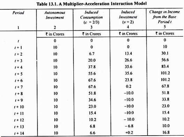
How the interaction between the multiplier and accelerator gives rise to the cyclical movements in economic activity (as measured by income or output) will become clear from Table 13.1. In formulating this table we have assumed that marginal propensity to consume (c) being equal to 2/3 or 0.66 and capital-output ratio (v) or accelerator being equal to 2.

Further, one period time-lag has been assumed which implies that an increase in income in a period induces the increase in consumption in the next period. It is assumed that initially in period t + 1, autonomous investment is of Rs. 10 crores.

In period t + 3, with autonomous investment being maintained constant at Rs. 10 crores, the deviation of total income in the period t + 3 as compared to the base period will be equal to 10 + 20 + 26.6 = Rs. 56.6 crores. Similarly, the changes in induced consumption and induced investment and hence in income brought about by the initial increase in autonomous investment of Rs. 10 crores which is maintained throughout, can be found out.

It will be seen from column 5 of Table 13.1 that there are large fluctuations in income. Under the influence of the interaction between the multiplier and accelerator, the income increases up to the period t + 6. In other words, period up to t + 6 represents the expansion phase or upswing of the business cycle.

Therefore, the period t + 6 is the upper turning point of the business cycle beyond which the contraction phase or downswing of the business cycle begins. It will be further observed that beyond the period t + 13, income again starts rising, that is, recovery from the depression begins. Thus, t + 13 represents the lower turning point of the business cycle.

In this way we see that the interaction between the multiplier and accelerator can give rise to the cyclical movements of the economic activity and its various phases. It is worth mentioning that we have taken particular values of marginal propensity to consume (which determine the size of the multiplier) and capital-output ratio (which determines the size of the accelerator). The other values of multiplier and accelerator that have been explained above would give rise to the different patterns of fluctuations.