Theory of Real Business Cycles and Economic Fluctuation

Theory of Real Business Cycles and Economic Fluctuation!

Introduction:

Most Economists believe that the classical model cannot explain the short- run economic fluctuations because in this model prices are flexible.

However the new classical economists believe that the classical model can explain the short-run economic fluctuations. They believe that it is best to assume that prices are flexible even in the short-run.

Almost all microeconomic analysis is based on the assumption that prices adjust to clear markets. New classical economists argue that macroeconomic analysis should be based on the same assumption. The leading new classical explanation of economic fluctuations is called the theory of real business cycles.

According to this analysis, the assumption that have been used for long-run may also apply for short-run study. Most importantly, real-business-cycle theory holds that the economy obeys the classical dichotomy nominal variables are assumed not to influence real variables. To explain fluctuations in real variables, real-business-cycle theory emphasis real changes in the economy, such as changes in fiscal policy and production technologies. This theory excludes the nominal variables to explain economic fluctuations.

Here we examine a simple theory of real business cycles.

A Review of the Economy under Flexible Prices:

The real-business-cycle theory is a new theory of fluctuations which requires the IS-LM model, under the assumption of flexibility of prices. We then modify it to develop a real model of short-run fluctuations.

In the IS-LM model we used the following equations for the goods and money markets:

Y = C (Y – T) + l(r) + G…………..  IS

M/P = L(r, Y)…………. LM

The first equation is the IS equation, which states that income Y is the sum of C, I, G consumption, depends on disposable income (Y – T) investment depend on the real interest rate, r, Govt. expenditure, G which is autonomous. The second equation is the LM equation which states that the supply of real money balances, M/P equals the demand, which is the function of the interest rate and the level of income. For simplicity we are assuming that expected inflation is zero, so that, the nominal interest rate equals the real interest rate.

To analyse the short-run fluctuations with the IS-LM model, we assume that price level is fixed. If prices are flexible, then the price level adjusts so that output is at its natural rate: Y = Y = F (K, L). These three equations determine three endogenous variables: the level of output Y, the real interest rate r, and the price level P.

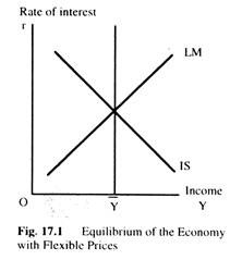
Fig. 17.1 shows the equilibrium of the economy with flexible prices. The level of output is at its natural rate y which is determined by the supply of factors of production and the production function. The interest rate is determined by the intersection of the is curve and the vertical line y the natural rate of output. The price level adjusts, so that the lm curve crosses the intersection of the other two curves.

It may be noted that the LM curve is not very important here as the prices are flexible and the price level adjusts to equilibrate the money market where the other two curves intersect. For the purpose of understanding the real variables, such as output and interest rate, we can ignore the money market.

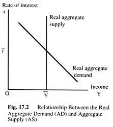
The two key relationships under flexible prices can be shown in Fig 17.2. These two relationships are real aggregate demand and real aggregate supply. The is curve is called here the real aggregate demand curve, which shows that the demand for goods and services is a function of the interest rate Real aggregate supply shows the supply of goods and services, which is determined by the supply of factors of production and the availability of technology.

In Fig. 17.2, the interest rate is on the vertical axis instead of price level as we have already seen in the case of aggregate demand and aggregate supply curves. In business-cycle theory, we are interested in real variables and not nominal variables, so the price level is unimportant. We are now developing a different theory of economic fluctuations.

A Real-Business-Cycle Model:

We now turn our model of the economy under flexible prices into a model of fluctuations. The new feature of the model is the behaviour of labour supply. In a classical model the supply of labour is fixed which determines the level of employment. Yet employment fluctuates over the business cycle. II we maintain classical assumption that labour market clears, as new classical economists do, then we must examine what causes fluctuations in the quantity of labour supplied.

After discussing the determinants of labour supply, we modify classical model, aggregate income to include changes in labour supply. The supply of output depends in part on the supply of labour, which means that the greater the number of hours people are willing to work, the more output the economy can produce. We examine how various events influence labour supply and aggregate income according to real-business-cycle theory.

Inter-Temporal Substitution of Labour:

Real-business-cycle theory states that the quantity of labour supplied depends on the incentives that workers receive at any point in time. When workers are well rewarded, they wish to work more hours, and vice versa. This willingness to reallocate hours of work over time is called the inter-temporal substitution of labour. For example, a second year college student has two years summer vacations left before graduation. He wishes to work for one of these summers and to relax during the other summer. How should he choose which summer to work?

Let W₁ be his real wage in the first summer, and W₂ the real wage he expects in the second summer. Choosing which summer to work means comparing these two wages. Since the student can earn interest on money earned earlier, money earned in the first summer is worth more than money earned in the second summer.

Let r be the real interest rate. If the student works in the first summer and saves his earnings, he will have (1 + r) W₁ a year later. If he works in the second summer, he will have W₂. The inter-temporal relative wage is (1 + r) W₁/W₂. Working in the first summer is more attractive if the interest rate is high or if the wage is high relative to wage expected to prevail in the future.

According to real-business-cycle theory, all workers calculate cost-benefit analysis to decide when to work and when to enjoy leisure. If the wage is temporarily high or if the interest rate is high, it is good time to work. If the wage is temporarily low or if the interest rate is low, it is a good time to enjoy leisure.

Real-business-cycle theory uses the inter-temporal substitution of labour to explain why employment and output fluctuate. Shocks to the economy that cause the interest rate to rise or the wage rate to be temporarily high cause people to want to work more—which raises employment and output.

Real Aggregate Demand and Real Aggregate Supply:

Real-business-cycle theory incorporates inter-temporal substitution of labour into the classical model of the economy. Our analysis of labour supply shows that the interest rate influences the attractiveness of working today.

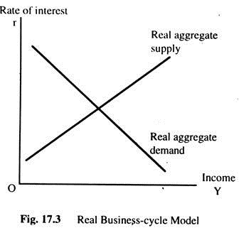
The higher the interest rate, the greater the amount of labour supplied, and the greater the amount of output produced. Fig. 17.3 shows the real-business-cycle model of the economy. Because of inter-temporal substitution of labour, the real aggregate supply curve slopes upward rather than vertically, which means a higher interest rate makes working more attractive, which increases labour supply and, thus, output.

The real interest rate adjusts to equilibrate real aggregate supply and real aggregate demand. We can use this model to explain fluctuations in output. Any shock to the economy that shifts aggregate demand or aggregate supply changes equilibrium output. Inter-temporal substitution of labour leads to a corresponding change in the level of employment as well.

To explain shifts in real aggregate demand and supply, real-business-cycle theorists have emphasised changes in fiscal policy and in technology. We now examine these sources of short-run fluctuations.

Fiscal Policy:

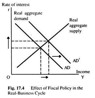
An increase in government purchases is shown in the real-business-cycle model. Fig. 17.4 shows an increase in government purchases shifts the real aggregate demand curve rightward. The result is higher output and a higher real interest rate.

It may be noted that there are similarities between this explanation of the effects of fiscal policy and the one we saw in the IS-LM model. An increase in government purchases shifts the real aggregate demand curve outwards for the same reason that it shifts the IS curve outwards in the IS-LM model. In both cases, the result is higher output and a higher interest rate. Thus, the two models make similar predictions.

However, there are important differences between the two explanations. In the IS-LM model, prices are stable, and aggregate demand determines output and employment; labour supply and inter-temporal substitution play no role in explaining how fiscal policy influences output.

In a real-business-cycle model, prices are flexible, and workers inter-temporally substitute labour. The expansion of output results from an increase in labour supply; people respond to the higher interest rate by choosing to work longer hours.

Technology:

Many theorists emphasise the role of shocks in technology. To see how technological shocks cause fluctuations, suppose some improvements in tech­nology are available, such as, faster computers. According to this theory, this change affects the economy in two ways.

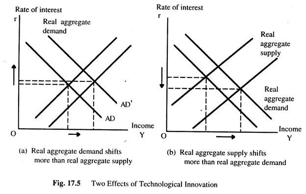
Firstly, the improved technology increases the supply of goods and services. As the production function is improved, more output is produced for any given input. The real aggregate supply curve shifts outwards.

Secondly the availability of the new technology rises the demand for goods. For example, firms wishing to buy these computers will raise their demand for goods. For example, firms wishing to buy these computers will raise their demand for investment goods. The real aggregate demand curve shifts outwards as well.

Fig. 17.5 shows two effects. A beneficial shock to the technology raises both real aggregate supply and real aggregate demand. In Fig. 17.5(a), demand shifts more than supply. In Fig. 17.5(b), demand shifts less than supply.

The Debate over Real-Business-Cycle Theory:

Economists disagree about the validity of real-business-cycle theory.

At the heart of the debate are four basic issues:

(a) The importance of technology shocks.

(b) The interpretation of unemployment.

(c) The neutrality of money.

(d) The flexibility of wages and prices.

(a) The Importance of Technological Shocks:

Real-business-cycle theory assumes that the economy experiences fluctua­tions in its ability to turn inputs into outputs, and that these fluctuations in technology cause fluctuations in output and employment. When the available production technology improves, the economy produces more output with the same inputs. Because of inter-temporal substitution of labour, the improved technology also leads to greater employment.

This theory often explains recessions as periods of technology regress. According to this theory, output and employment fall during recessions because the available production technology deteriorates, which reduces output and the incentive to work.

Critics of this theory are sceptical that the economy experiences large shocks in technology. It is common knowledge that technological progress takes place gradually. It is difficult to think that technology can regress. The technological knowledge may slow down, but it is hard to imagine that it would go into reverse.

Advocates respond by taking a broad view of shocks to technology. They argue that there are many events that—although not literally technological in nature—nevertheless, affect the economy as much as technological shocks do. For example, bad weather or increases in world oil prices have effects similar to adverse changes in technology. Whether such events are sufficiently common to explain the frequency and magnitude of business cycles is open to question.

(b) The Interpretation of Unemployment:

Real-business-cycle theory assumes that fluctuations in employment reflect changes in the amount people want to work. Alternatively, it assumes that the economy is always on the labour supply curve: everyone who wants a job at the going wage rate can find one. To explain fluctuations in employment, advocates of this theory argue that changes in wage rates and interest rates cause inter-temporal substitution of labour.

Critics of this theory believe that fluctuations in employment do not reflect changes in the amount people want to work. They do not think desired em­ployment is very sensitive to real wage and the real interest rate. They point out that unemployment fluctuates substantially over the business cycle.

The high unemployment in recessions suggests that the labour market does not clear: if people were voluntarily choosing not to work in recessions, they are not, in fact, unemployed. These critics conclude that, wages do not adjust to equilibrate labour demand and supply, as the real-business-cycle model assumes.

Advocates of this theory argue that unemployment statistics are difficult to interpret. The mere fact that the unemployment rate is high does not mean that inter-temporal substitution of labour is unimportant. Individuals who voluntarily choose not to work may call themselves unemployed to received unemployment benefits. Alternatively; they may call themselves unemployed because they would be willing to work.

(c) The Neutrality of Money:

This theory assumes that money is neutral which means monetary policy is assumed not to affect real variables, such as output and employment. The neutrality of money not only gives this theory its name, it is also the most radical feature of the theory.

Critics point out that the evidence does not support the assumption of neutrality of money. They argue that reductions of money growth and inflation are always associated with periods of high unemployment. Monetary policy appears to have a strong influence on the real economy.

Advocates of the theory argue that their critics confuse the direction of causation between money and output. They also claim that money supply is endogenous: fluctuation in output might cause fluctuations in money supply.

For example, when output rises—because of beneficial technological shock— the quantity of money demanded rises. The central bank may respond by raising money supply to accommodate the greater demand. This endogenous response of money to economic activity may give the illusion of non-neutrality of money.

(d) The Flexibility of Wages and Prices:

Real-business-cycle theory assumes that wages and prices adjust quickly to clear markets. Proponents of this theory believe that the stickiness of wages and prices is unimportant for understanding economic fluctuations. They also believe that the assumption of flexible prices is methodologically superior to the assumption of sticky prices, because it ties microeconomic theory to macroeconomic theory more closely.

Most of microeconomic analysis is based on the assumption that prices adjust quickly to equate demand and supply. Advocates of this theory believe that macroeconomists should base the analysis on the same assumption. Critics argue that money wages and prices are inflexible—which explains both the existence of unemployment and monetary non-neutrality. To explain stickiness of prices, they rely on the various new Keynesian theories.

Conclusion:

Real-business-cycle theory reminds us that our understanding of economic fluctuations is not good enough. Fundamental questions about the economy remain open to dispute. Is the stickiness of wages and prices a key to our understanding of economic fluctuations? Does monetary policy have real ef­fects?

The way economists answer these questions influence the way they view the role of the economic policy. Those who believe that wages and prices are sticky often believe that fiscal and monetary policy should be used to try to stabilise the economy. Price stickiness is a type of market imperfection, which leaves open the possibility that government policies can raise economic benefits.

By contrast, the theorists believe that the government’s ability to stabilise the economy is limited. They view the business cycle as the efficient and natural response of the economy to technological changes. Most models of this theory do not include any market imperfection and believe that the invisible hand guides the economy to an optimal allocation of resources. These two views of economic fluctuations are a source of frequent and heated debate. It is this kind of debate that makes macroeconomics an attractive field of study.

Long-Run Economic Fluctuations:

Cyclical fluctuations in the level of economic activity can be observed by examining annual changes in real national income over a long period of years. These changes are inversely related to variations in the rate of unem­ployment. The fluctuations were much reduced, possibly as a result of the adoption of Keynesian demand management policies by all governments in the developed capitalist economies since 1950s.

None the less, even in this period, the economy has been subjected to fairly regular cycles of minor expansions and recessions. In the 1970s, the business cycle was marked by world recession—due to the energy crisis—which resulted in an upward trend in the rate of unemployment.

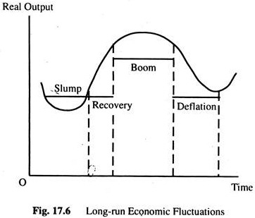
The phases of the business-cycle-slump, recovery, boom and deflation — are illustrated in Fig. 17.6. An economy in a slump is experiencing high demand- deficient unemployment of both labour and capital. A low level of both investment and consumption demand leads firms to cut back on their production, lay off workers and leave capital goods idle. Although money may be available for firms to borrow and interest rates may be low, investment will not increase because of pessimistic expectations.

In the recovery phase the level of aggregate demand is rising and, thus, businessmen become more optimistic. Generally, this is a period of rising consumer demand, investment demand, expanding output levels and a falling rate of unemployment. Eventually, the economy reached a boom period. This is a time of low unemployment, a high level of demand, high level of output and profits, an increasing rate of inflation and rising interest rates.

Finally, in the deflation phase, the demands of both firms and households start to fall, firms’ profits dwindle and output and employment levels are reduced. Again, businessmen become pessimistic about the future level of demand for their product and so become extremely reluctant to invest in new capital, even for replacement purposes.

Ultimately, this contracting economy reaches the slump again and the whole process is repeated. The objective here is to consider the possible causes of this cyclical movement in economic activity. We concentrate on the multiplier-accelerator theory to explain the fluctuations.

Multiplier-Accelerator Interaction:

Samuelson’s trade cycle theory is based on the interaction between the multiplier process and the accelerator principle. This model concentrates on the real sector of the economy and so excludes monetary variables.

According to the ‘accelerator’ principle, investment depends on changes in income, and according to the multiplier, changes in investment cause changes in income. Thus, it is natural that interaction between the two can result in cumulative movements in income— for example, if income is rising at an increasing rate, both investment and consumption will be rising, causing further rises in income in the next period. A turning point may be reached if income increases at a decreasing rate; investment will start to fall and as soon as the fall in investment exceeds the rise in consumption, income will start to fall as well.

The following assumptions are sufficient to generate a cyclical movement in national income after an exogenous change in investment or consumption has taken place:

(1) The consumption function is lagged by one period which means that consumption in the current period depends on the national income in the previous period. That is, C_t = cY_{t – 1}, where c is both the marginal and average propensity to consume.

(2) The accelerator is such that, induced investment depends on the difference between national income in the last period and in the period before that. Thus, we can write, I_t = I₀ + ν (Y_{t – 1} – Y_{t – 2}) where I₀ is exogenous investment and u is the accelerator.

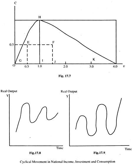
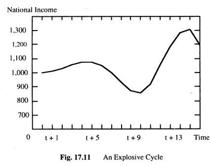
(3) The values of v and c must lie below the curve shown in Fig. 17.7. For example, if the values of c and u lie in the area GHJ (say c = 0.5 and u = 0.5) as at point E, then any exogenous change in consumption or investment will generate a damped cycle like that given in Fig. 17.8; it is called damped, because the fluctuations in real output become smaller and smaller over time. But if the values of c and v lie in the area JHK ( for example, c = 0.5 and v = 1.5 at point F) then any exogenous change in spending will generate an explosive cycle like that, in Fig. 17.9; here the oscillations get larger and larger over time.

There may be various types of cycle between these two extremes depending on values of c and v.

The derivation of the curve-in Fig. 17.7 is beyond the scope of this book. However, we can partially demonstrate its validity by means of two simple numerical examples.

Example 1:

A Damped Cycle:

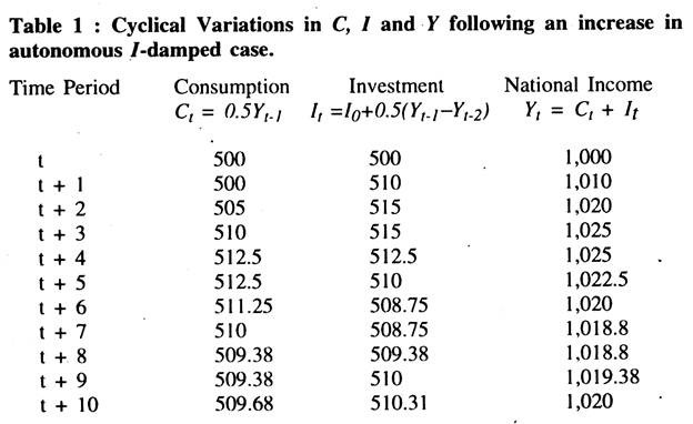
To simplify our analysis, we consider a closed economy without a government, so that, Y = C + I. Suppose, for the last several periods of time, real national income has been constant at £1,000. Let c = 0.5 and v= 0.5 (as at Point E in Fig. 17.7) and suppose, initially autonomous investment do) = £500, we have, C_t = 0.5 Y_{t – 1} = £ 500.

I_t = 500 + 0.5 (Y_{t – 1} – Y _{t – 2}) = £500

Y_t = C_t + I_t = 500 + 500 = £1.000

The economy is in equilibrium in the current period, t. Suppose that, in the next period of time t + 1, autonomous investment, I₀, rises by £10 to £510. Now we have, Y _{t + 1} = C _{t + 1} + l _{t + 1} = 500 + 510 = £1,010. This rise in income from period t to period t + 1 will cause both consumption and investment in the next period, t + 2, to rise:

C _{t + 1} = 0.5Y _{t + 1} = £505

I _{t + 1} = 510 + 0.5 (Y _{t – 1} – Y_t) = 510 + 5 = £515.

This means that, Y_{t + 2} = C_{t + 2} + l_{t + 2} = 505 + 515 = £1,020.

This further rise in income from period t + 1 to t + 2 will cause C and I in period t + 3 to rise again.

C_{t + 3} = 0.5Y_{t + 2} = £510

I _{t + 3} = 510 + 0.5 (Y_{t + 2} – Y_{t + 1}) = 510 + 5 + £515

.^.. Y _{t + 3} = 510 + 5/5 = £1.025 and so on in subsequent periods.

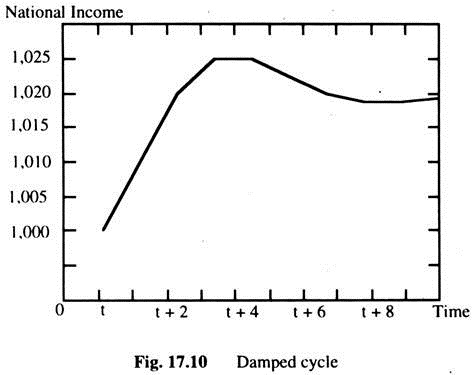
So far in the analysis, the single increase in autonomous investment of £10 has caused income to rise from £1,000 to £1,025 in the first four time periods and then start to fall in the fifth. Taking the little time-path to period t + 10, we obtained a clearly damped cyclical variation in real national income. This is summarised in Table 1 and Fig. 17.10.

It may be noted that eventually the cycle will converge on the new equilibrium level of income of £1,020 (since the multiplier is 2 in this example). Only when income settles at £1,020 can we say that, the full multiplier effect has taken place. However, no new equilibrium position is likely to reach in the case of an explosive cycle, as is shown in the next example.

Example II:

An Explosive Cycle:

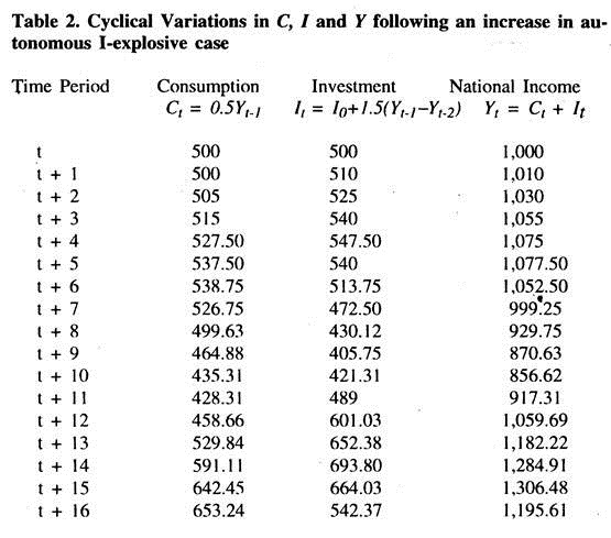
Now suppose c=0.5 and v = 1.5 (point Fin Fig. 17.7). Assume, as before, that Y has been constant for several time periods at £1,000, and the autonomous I is equal to £500. This means that the economy is in equilibrium in period t. Now suppose, autonomous I rises to £510 in period t + 1. This rise in spending will raise Y to £1010 in period t + 1 and this will cause both C and I to increase in the next period, t + 2: C_t+2 = 0.5Y_t+1 =£505 I_t+2 = £510 + 1.5(Y_{t + 1} – Y_t) = 510 + 15 = £525.

Therefore, Y_t+2 = 505 + 525 = £1,030

It may be noted that I and Y have already risen above the levels reached in the previous example. The time-path to period t +16 is given in Table 2 and Fig. 17.11. An explosive cyclical variation in national income, Y, results. Although the arithmetic becomes quite laborious, but it is a worthwhile exercise.

Ceilings and Floors:

We have seen that the multiplier-accelerator model is capable, under certain circumstances, of generating cycles automatically following any change in autonomous spending. Depending on the values assigned to c and v, the cycle may be damped and explosive. Table 1 shows that, cycle in practice displays no obvious tendency either to diminish or increase in amplitude over time, but in the 19th century, the amplitude of the cycle was remarkably constant.

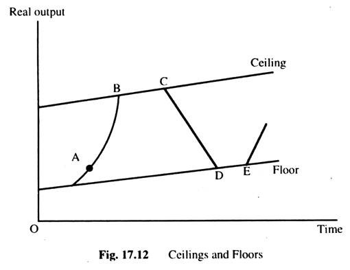
A possible explanation is that the cycle is inherently explosive, but is constrained within a band determined by an upper limit, called a ceiling and lower limit, called a floor. The cycle thus generated will tend to have a constant amplitude determined by ceiling and floor. Such a cyclical movement in real output is illustrated in Fig. 17.12.

To explain how such a movement will develop, start at point A in Fig. 17.12. This is in the recovery phase. Consequently, demand is increasing, output is expanding and unemployment is falling. In terms of the multiplier-accelerator interaction, rising investment will cause Y to rise via the multiplier effect and the rising level of Y induces more investment to occur via the accelerator. Soon full employment will be reached (point B in Fig. 17.12) which determine the ceiling because now real output can only rise as net new investment comes into operation.

Firms may want to produce more at point B but are unable to do so, because of insufficient resources. This check to the growth of output and income will soon affect firms’ investment plans via the accelerator. In fact, since the increase in income has slowed down, induced investment will actually fall and this causes income itself to fall via the multiplier. The existence of the ceiling brings about a turning-point and after point C, real output starts falling.

Real output will continue to fall with multiplier-accelerator interacting with each other until the floor is reached. What determine the position of the floor? As we know, income cannot fall below zero, so that represents an absolute floor. However, investment demand can fall to zero when firms are so pessimistic that they have no demand for either new or replacement capital. Consumption demand must always be positive, if to sustain life. This consumption spending must represent floor below which the level of income cannot be expected to fall.

Furthermore, it is likely that some investment will always occur somewhere in the economy, so that aggregate investment can never fall to zero. Once point D has been reached, output will have stopped falling and, eventually, some replacement investment will become unavoidable. This will set the multiplier-accelerator interaction into operation again.

The existence of the floor brings about another turning point, so that, after point E is reached, real output starts rising again. This brings us back to the recovery phase and the whole process starts again. Notice that, each peak and trough is likely to be above all preceding ones because of underlying growth in the economy’s productive capacity.

Random Disturbances:

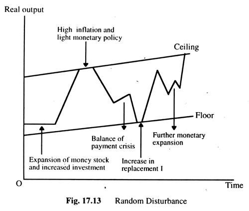
The existence of ceilings and floors can help to explain the regularity of cycles, but without c and v constraints, the cycles could be explosive. Suppose c and v took on values consistent with damped cycles, how then could we explain the observed regularity of cyclical fluctuations?

One possible answer has been suggested by R. Frisch, who argues that, even though fluctuations around the equilibrium growth path are damped, random disturbances will be occurring continuously to stop the equilibrium path from being achieved and to maintain the cyclical variations in a fairly regular pattern.

No sooner has one cycle started to diminish in amplitude than another disturbance occurs, starting off a new cycle. The types of disturbances which could do this are changes in investment, balance of payment, crisis, changes in money supply, rapid inflation and policies designed to curb it, industrial disputes, and so on.

Of course, it is possible for more than one disturbance to occur at the same time, thus lengthening the inherently damped cycle. This means that the ‘ceiling’ and ‘floor’ analysis may become relevant here as well as in the explosive cycles case. Random disturbances are shown in Fig. 17.13, which give rise to fairly realistic variations in real output.

In this kind of model, real output is volatile, reaching occasionally the ceiling or floor, with each successive random disturbance pushing real income downwards or upwards and with underlying stabilizing influences of the multiplier and accelerator.

Monetary Influences:

One of the random disturbances mentioned was a change in the money supply. We now consider to what extent changes in monetary variables may be responsible for cyclical variations in real output. We know that the monetarists put a great deal of faith in the correlation between changes in the money supply and changes in national income; especially in the study by Friedman and Schwartz emphasises the observation that all major recessions have been preceded by a fall in the money supply and all major inflations by excess money supply. They concluded that the monetary changes were not associated with changes in national income, but the change in the money supply that causes the change in national income.

Non-monetarists also recognise the role of money supply in real output, though they do not assign them such a major role as the monetarists. For example, they recognise that, in the recovery phase of the cycle, the demand for money will increase. If the increased money demand is not accommodated, interest rates will rise this will discourage investment and so contribute to the slowing down in the growth of output and consequently lead to the upper turning-point.

Similarly, in the deflationary phase, the money demand will be falling. If the money supply does not fall, interest rates will fall and, thus, encouraging new investment. This will contribute to the lower turning-point. However, its effectiveness depends on the interest-elasticity of investment which is like to be very low in the boom and slump periods of the cycle.