Notes on Convex Indifference Curves and Corner Equilibrium

When a consumer’s preferences are such that he likes to consume some amount of both the goods, he reaches an equilibrium position at the point of tangency between the budget line and his indifference curve.

This equilibrium position at the point of tangency which lies within commodity space between the two axes is often called interior solution.

The economic implication of the interior solution is that consumer’s pattern of consumption is diversified that is, he purchases some amount of both the commodities. Our knowledge of the real world tells us that consumers’ pattern of consumption is quite diversified and they often buy a basket or bundle of several different goods instead of spending their entire income on a single commodity.

In the context of two commodity model which is generally assumed in indifference curve analysis, assumption of diversification in consumption and an interior solution, which imply that consumer purchases some amount of both goods, is correct.

However, in the real world o many commodities we often find that a typical consumer does not buy positive amounts of a the goods and services available in the market. In fact, a typical consumer buys only a small number of goods available in the market. How to explain this real world phenomenon?

Convex Indifference Curves and Corner Equilibrium:

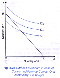
The reason for not purchasing a commodity by a consumer may be that the price or opportunity cost of that particular commodity may be too high for him. One may like to have Maruti car, air conditioner or a colour TV, but may not actually have it on account of their prices being too high. The indifference curve analysis enables us to explain even this phenomenon. Consider Figure 8.22 where indifference map between two goods X and Y and budget line BL are such that the interior solution is not possible and consumer in its equilibrium position at point B will not consume any quantity of commodity X.

This is because as seen in the Figure 8.22 the price of commodity X is so high that budget line is steeper than the indifference curves between the two commodities. In economic terms it means that the price or opportunity cost of commodity X in the market is greater than the marginal rate of substitution of X for Y which indicates willingness to pay for the commodity X.

The price of good X is so high as compared to marginal rate of substitution (willingness to pay for X or the marginal valuation of the first unit of the commodity X that the consumer does not purchase even one unit of the commodity X(P_x/P_y > MRS_y). Thus the consumer maximises his satisfaction or is in equilibrium at the corner point B where he buys only commodity Y and none of commodity X. Thus we have a corner solution for consumer’s equilibrium.

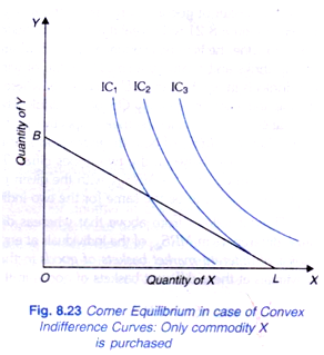
On the other hand, in Figure 8.23. the indifference map between the two goods is such that the budget line BL is less steep than the indifference curves between the two goods so that the MRS_y > P_X/P_y for all levels of consumption along the budget line BL. Therefore, he maximizes his satisfaction at the corner point L where he buys only commodity X and none of Y. In this case price of commodity Y and willingness to pay (i.e. MRS) for it are such that he does not consider it worthwhile to purchase even one unit of it.

Corner Equilibrium and Concave Indifference Curves:

The indifference curves are usually convex to the origin. Convexity of indifference curves implies that the marginal rate of substitution of X for Y falls as more of X is substituted for Y. Thus, indifference curves are convex to the origin when principle of diminishing marginal rate of substitution holds good and which is generally the case.

But the possibility of indifference curves being concave to the origin cannot be ruled out in some exceptional cases. Concavity of the indifference curves implies that the marginal rate of substitution of X for y increases when more of X is substituted for Y.

It will be clear from the analysis made below that in case of indifference curves being concave to the origin the consumer will choose or buy only one good. In other words, concavity of indifference curves implies that the consumer has a distaste for variety, that is, does not like diversification in consumption. However, distaste for variety cannot be considered a normal or model behaviour, so we regard convexity to be the general case. But when consumers have a distaste for variety and diversification the case of concave indifference curves will occur.

In case of concave indifference curves, the consumer will not be in equilibrium at the point of tangency between budget line and indifference curve, that is, in this case interior solution will not exist. Instead, we would have corner solution for consumer’s equilibrium. Let us take Fig. 8.24 here indifference curves are shown to be concave. The given budget line BL is tangent to the indifference curve IC₂ at point Q.

But the consumer cannot be in equilibrium at Q since by moving along the given budget line BL he can get on to higher indifference curves and obtain greater satisfaction than at Q. Thus by moving to K on the given budget line BL, he will get more satisfaction than at Q since K lies on a higher indifference curve than Q. He can increase his satisfaction still more by moving to point Z on the budget line BL.

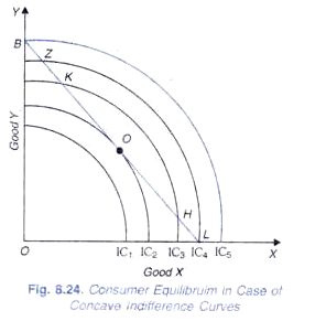
Thus, as he moves upward from tangency point Q on the budget line his satisfaction will go on increasing until he reaches the extremity point B. Likewise, if from Q he moves downward on the budget line, he will get on to higher indifference curves and his satisfaction will go on increasing till he reaches the other extremity point L.

In these circumstances the consumer will choose only one of two goods: he will buy either X or Y depending upon whether L or B lies on the higher indifference curve. In the situation depicted in Fig 8.24 point B lies on a higher indifference curve than point L. Therefore, the consumer will choose only Y and will buy OB of Y. It should be carefully noted that at B the budget line is not tangent to the indifference curve IC₅, even though the consumer is here in equilibrium. It is clear that when a consumer has concave indifference curves, he will succumb to monomania, that is, he will consume only one good.

Conclusion:

In our analysis above, we have shown that corner solution of consumer s equilibrium is possible even when his indifference curves between goods are convex. It is worth noting that in case of convex indifference curves, corner equilibrium is however not inevitable, it occurs only when price of a commodity is too high as compared to the marginal rate of substitution of even the first unit of the commodity.

However, when the indifference curves are concave consumer’s equilibrium will inevitably be a corner solution. This implies that more of commodity X a consumer has the more useful or significant in terms of satisfaction an extra unit of it becomes. Therefore, the concave indifference curves do not seem to be plausible or realistic.

Now, as seen above, the concavity of indifference curves for a consumer implies that the consumer spends his entire income on a commodity and therefore buys only one commodity. However, consumption of one good only by a consumer which the concavity of indifference curves leads us to believe is quite unrealistic. Observations in the real world reveal that consumers do not spend their entire income on a single commodity and in fact purchase a multitude of different goods and services. This rejects the existence of concave indifference curves.

Our analysis of inevitability of corner equilibrium in case of concave indifference curves provides us an important economic rationale for indifference curves being convex rather than concave. If indifference curves were predominantly concave the consumers would spend their entire income on a single commodity alone and thus consume only one commodity. This is quite inconsistent with the observed behaviour of consumers. This reinforces our belief that indifference curves of consumers are generally convex.

Corner Solution in Case of Perfect Substitutes and Perfect Complements:

Another case of corner solution to the consumer’s equilibrium occurs in case of perfect substitutes. As seen above, indifference curves for perfect substitutes are linear. In their case too, tangency or interior solution for consumer’s equilibrium is not possible since the budget line cannot be tangent to a point of the straight-line indifference curve of substitutes.

In this case budget line would cut the straight-line indifference curves.

Two possibilities can be visualized:

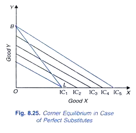
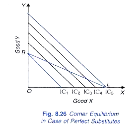
either the slope of the budget line BL can be greater than the slope of indifference curves, as in Fig. 8.25 or the slope of the budget line can be less than the slope of indifference curve, as in Fig. 8.26.

 

 

If the slope of the budget line is greater than the slope of indifference curves, B would lie on a higher indifference curve than L and the consumer will buy only Y. If the slope of the budget line is less than the slope of indifference curves, L would lie on a higher indifference curve than B and the consumer will buy only X.

It should be noted that in these cases too, the consumer will not be in equilibrium at any point between B and L on the price line since in case of Figure 8.25 of all the points on the given budget line extremity point B would lie on the highest possible indifference curve and in case of Figure 8.26 of all the points of the budget line extremity point L would lie on the highest possible indifference curve. It is thus manifest that even in case of perfect substitutes, the consumer will succumb to monomania.

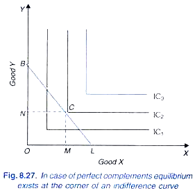
Another non-normal case is of perfect complementary goods, is depicted to Figure 8.27. Indifference curves of perfect complementary goods have a right-angled shape. In such a case the equilibrium of the consumer will be determined at the corner Fig.8.27.

In case of perfect complements equilibrium point of the indifference curve IC₂ which is indifference curve just touching the budget line BL at point C Indifference curve IC₂ is the highest possible indifference curve to which the consumer can go. In Figure 8.27, given the budget line BL the consumer will be in equilibrium at point Con indifference curve IC₂ and will be consuming OM of X and ON of Y.