Price Leadership (With 3 Forms and Diagrams)

Another form of collusion is price leadership. In this form of coordinated behaviour of oligopolists one firm sets the price and the others follow it because it is advantageous to them or because they prefer to avoid uncertainty about their competitors’ reactions even if this implies departure of the followers from their profit-maximizing position.

Price leadership is widespread in the business world. It may be practiced either by explicit agreement or informally. In nearly all cases price leadership is tacit since open collusive agreements are illegal in most countries.

Price leadership is more widespread than cartels, because it allows the members complete freedom regarding their product and selling activities and thus is more acceptable to the followers than a complete cartel, which requires the surrendering of all freedom of action to the central agency. If the product is homogeneous and the firms are highly concentrated in a location the price will be identical. However, if the product is differentiated prices will differ, but the direction of their change will be the same, while the same price differentials will broadly be kept.

There are various forms of price leadership.

The most common types of leadership are:

(a) Price leadership by a low-cost firm.

(b) Price leadership by a large (dominant) firm.

(c) Barometric price leadership.

These are the form of price leadership examined by the traditional theory of leader­ship as developed by Fellner and others. The characteristic of the traditional price leader is that he sets his price on marginalistic rules, that is, at the level defined by the intersection of his MC and MR curves. For the leader the behavioural rule is MC = MR. The other firms are price-takers who will not normally maximise their profit by adopting the price of the leader. If they do, it will be by accident rather than by their own in­dependent decision.

 

A. The Model of the Low-cost Price Leader:

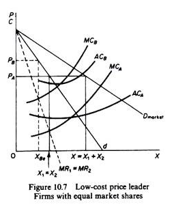
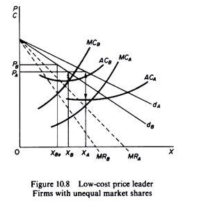
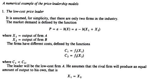
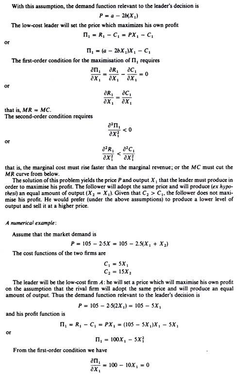
We will illustrate this model with an example of duopoly. It is assumed that there are two firms which produce a homogeneous product at different costs, which clearly must be sold at the same price. The firms may have equal markets (or they may come to an agreement to share the market equally) as in figure 10.7, or they may have unequal markets (or agree to share the market with unequal shares), as in figure 10.8. The important condition for this model is that the firms have unequal costs.

The firm with the lowest cost will charge a lower price (P_A) and this price will be fol­lowed by the high-cost firm, although at this price firm B (the follower) does not maximize its profits. The follower would obtain a higher profit by producing a lower output (X_Be) and selling it at a higher price (P_B). However, it prefers to follow the leader, sacrificing some of its profits in order to avoid a price war, which would eliminate it if price fell sufficiently low as not to cover its LAC. It should be stressed that for the leader to maximize his profit price must be retained at the level P_A and he should sell X_A. This implies that the follower must supply a quantity (0X_B in figure 10.8, or OX₁ = OX₂ in figure 10.7) sufficient to maintain the price set by the leader.

Although the price- leadership model stresses the fact that the leader sets the price and the follower adopts it, it is clear that the firms must also enter a share-of-the-market agreement, formally or informally, otherwise the follower could adopt the price of the leader but produce a lower quantity than the level required to maintain the price (set by the leader) in the market, and thus push (indirectly, by not producing enough output) the leader to a non-profit-maximising position.

In this respect the price follower is not completely passive he may be coerced to adopt the leader’s price, but, unless tied by a quota-share agreement (formal or informal) he can push the leader to a non-maximising position.

B. The model of the Dominant-firm Price Leader:

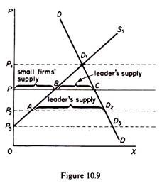
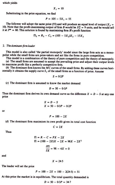
In this model it is assumed that there is a large dominant firm which has a considerable share of the total market, and some smaller firms, each of them having a small market share. The market demand (DD in figure 10.9) is assumed known to the dominant firm.

It is also assumed that the dominant leader knows the MC curves of the smaller firms, which he can add horizontally and find the total supply by the small firms at each price; or at best that he has a fair estimate, from past experience, of the likely total output from this source at various prices. With this knowledge the leader can obtain his own demand curve as follows.

At each price the larger firm will be able to supply the section of the total market not supplied by the smaller firms. That is, at each price the demand for the product of the leader will be the difference between total D (at that price) and the total S₁. For example, at price P₁ the demand for the product of the leader will be zero, because the total quantity demanded (D₁) is supplied by the smaller firms.

As price falls below P₁ the demand for the leader’s product increases. At P₂ the total demand is D₂; the part P₂ A is supplied by the small firms and the remaining AD₂ is supplied by the leader. At P₃ total demand is D₃ and the total quantity is supplied by the leader since at that price the small firms do not supply any quantity. Below P₃ the market demand coincides with the leader’s demand curve.

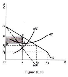
Having derived his demand curve (d_L in figure 10.10) and given his MC curve, the dominant firm will set the price P at which his MR = MC and his output is 0x. At price P the total market demand is PC, and the part PB is supplied by the small firms followers while quantity BC = 0x is supplied by the leader.

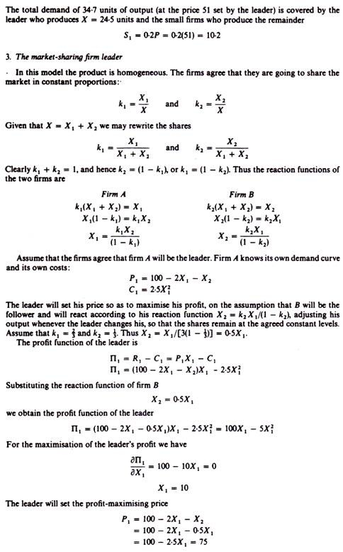
The dominant firm leader maximises his profit by equating his MC to his MR, while the smaller firms are price-takers, and may or may not maximise their profit, depending on their cost structure. It is assumed that the small firms cannot sell more (at each price) than the quantity denoted by S₁. However, if the leader is to maximise his profit, he must make sure that the small firms will not only follow his price, but that they will also produce the right quantity (PB, at price P). Thus, if there is no tight sharing-the- market agreement, the small firms may produce less output than PB and thus force the leader to a non-maximising position.

C. Barometric Price Leadership:

In this model it is formally or informally agreed that all firms will follow (exactly or approximately) the changes of the price of a firm which is considered to have a good knowledge of the prevailing conditions in the market and can forecast better than the others the future developments in the market. In short, the firm chosen as the leader is considered as a barometer, reflecting the changes in economic environment.

The baro­metric firm may be neither a low-cost nor a large firm. Usually it is a firm which from past behaviour has established the reputation of a good forecaster of economic changes. A firm belonging to another industry may also be chosen as the barometric leader. For example, a firm in the steel industry may be agreed as the (barometric) leader for price changes in the motor-car industry. Barometric price leadership may be established for various reasons.

Firstly, rivalry between several large firms in an industry may make it impossible to accept one among them as the leader. Secondly, followers avoid the continuous recalculation of costs, as economic conditions change. Thirdly, the barometric firm usually has proved itself as a ‘reasonably’ good forecaster of changes in cost and demand conditions in the particular industry and the economy as a whole, and by following it the other firms can be ‘reasonably’ sure that they choose the correct price policy.