The following article will guide you about how to construct a customer’s income and price consumption curve.
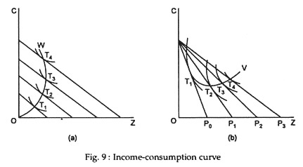
If the income of the consumer increases, his budget line will have the same slope (relative price ratios remaining unchanged) but that line will then shift to the right (he can get more goods for his increased money income). Thus, income changes will cause parallel shifts of the budget line and a set of parallel budget lines [Fig. 9(a)] shows how the consumer’s desired purchase is likely to vary with changes in his income.
On each such line we can find the equilibrium point of tangency (points T1, T2, etc.). The curve OW, which is the locus of all such equilibrium points, shows how the consumer’s purchases of the two commodities will vary when his income changes. Such a curve is called an income-consumption curve, also known as an Engel curve. It shows the reaction of the consumer to income changes.
ADVERTISEMENTS:
In case of normal goods, consumers are found to increase their purchases of commodities as their incomes rise. But, sometimes, if an item is of low quality, demand for it will fall as the consumer’s economic condition improves and more desirable commodities are substituted for it. Such an item is called an inferior good, such as recapped automobile tires, poorly made clothing, poor quality of rice etc., any of which the consumer may be buying only because he can afford no better.
In Fig. 9(a) commodity Z is assumed to be an inferior good. Points T3 and T4 (the negatively sloping segment of OW) clearly reveal this. The latter point lies to the left of the former (it represents a lower quantity of Z) notwithstanding the fact that it (T4) is on a higher budget line and therefore involves a higher money income for the consumer. In this case Z is an inferior good and C is a superior good.
Thus, if the consumer spends all his income on just two commodities both cannot be inferior at the same time. If both C and Z are inferior, the consumer will be left with some unspent income. Obviously, he will have to operate inside the budget line by moving downward from T3 to T2 rather than moving upward from T3 to T4.
We may now examine the effects on the consumer’s purchases of changes in the price of one of the purchasable commodities. Let us suppose the price of Z falls, other things remaining unchanged. The implication is that the buyer can get more of this commodity with the same amount of money income [e.g., OP1 instead of OP0 in Fig. 9(b)], though he can only acquire the same amount of C as before (i.e., OP0). We see then that a fall in the price of the item on the horizontal axis makes the budget line flatter.
ADVERTISEMENTS:
Fig. 1(b) represents a number of such budget (price) lines and the corresponding equilibrium points. Curve PV, the locus of these points of tangency, shows the reaction of the consumer to changes in the price of Z. In fact, a change in the price of Z will affect the purchases of both commodities. Here PV is called a price-consumption curve which is also derived from the indifference map of the consumer.
One may note that the income-consumption curve, OW, starts from the origin (point O) because with zero income the consumer can buy none of either commodity. Contrarily, the price-consumption curve, PV, characteristically begins at point P, the pivot point of the swinging price line in Fig. 9(b).
The reason is easy to find out — as the price line approaches the vertical axis (the price of Z increases further and further), the consumer finds that he get less and less of Z with his income. Eventually, when its price goes up to a very high level, the consumer will be forced to stop buying Z altogether and he will therefore spend all his income on the remaining commodity, C, i.e., he will buy OP units of C and no Z (point P).

