Conditions for Consumer Equilibrium | Microeconomics

In this article we will discuss about the conditions for consumer equilibrium.

1. Consumer Equilibrium – Single Commodity Case:

Now see how the consumer buying a single good in the market, would behave.

Let’s assume:

(i) The purchase would be confined to only one commodity.

(ii) The price of the commodity is given in the market. The consumer only determines how much to buy at the given price.

(iii) The consumer is a rational human being and, as such, his goal is to maximise the consumer’s surplus which means the surplus of utility he earns over his expenditure on the good at the point of purchase.

(iv) There are no constraints on the consumer’s expenditure, i.e., he has sufficient money to buy whatever quantity he decides to buy to achieve his goal.

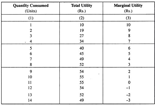
Now concentrate on the logic upon which the consumer’s behaviour will be based. Refer to Table 5.1 where a consumer’s hypothetical TU and MU data have been given.

Table 5.1. Total and Marginal Utility Schedule of a Consumer in the Consumption of a Particular Good

Suppose that the price of the good is given to be Rs 7 in the market. Now the question is how much of the good the consumer will decide to buy. Let’s proceed in this way. The consumer will buy the first unit because he derives a marginal utility of Rs 10 from this unit whereas he would have to pay Rs 7 only as its price, i.e., he gains an excess or surplus of Rs 3 of utility over the amount he pays.

In the same way, the consumer will decide to buy the second unit, for he gets a marginal utility of Rs 9 from this unit whereas he has to pay Rs. 7 only as its price, i.e. now he gains surplus of Rs 2 of utility over the amount he pays as price.

Now, since at q = 2, the MU has been greater than price, he would proceed to buy the third unit by the same logic. In other words, so long as MU > p, the consumer would decide to increase his purchase of the good. But, as q increases, MU would fall monotonically because of LDMU and, at some q, it would come down to the level of the price of the good, which is given and constant.

In the example, at q = 4, MU has diminished to the level of p = 7 (Rs). It may be noted that for the 4th unit, MU – p = 0, and the consumer is not able to have any surplus utility over the price when he buys the 4th unit. For all the earlier units, as seen, he has earned some surplus.

However, the consumer would not proceed to buy the 5th unit for, at q = 5, MU = Rs 6 < p = Rs. 7, i.e., now the price the consumer pays for the 5th unit exceeds the MU he gains, i.e., now he would have a negative surplus (= − Re 1) from the 5th unit.

What is obtained, a rational consumer would go on increasing the quan­tity to be purchased of a good so long as MU > p, i.e., so long as he expects to earn a positive surplus on the marginal unit, and, as he increases the quantity, the (marginal) surplus would be falling because of the LDMU and, at some q, it would fall to zero.

At that point, he would stop increasing his purchase, because if he increased his purchase beyond that point he would earn a negative surplus on the margin.

In other words, in the case of a single commodity purchase, the consumer equilibrium would be obtained at a point where surplus on the marginal unit is zero and where his total surplus obtained, is maximum. This maximum surplus obtained at the equilibrium point of the consumer is known as the consumer’s surplus.

Consumer’s Surplus—Formal Definition:

Now give the formal definition of consumer’s Surplus which is defined at the point of his purchase.

Consumer’s Surplus = total utility obtained – total expenditure

(at the consumer’s equilibrium point)

= total utility – price x quantity purchased

= total utility – marginal utility x quantity purchased

In the example, when the price of the good is Rs 7, the consumer would be in equilibrium, i.e., he would have the maximum surplus, if he buys 4 units of the good. At q = 4, then:

Consumer’s Surplus = 34 – 7 x 4 (Rs)

= 6 (Rs)

This is the maximum amount of surplus that the consumer would be able to earn from his purchase of the good at p = 7 (Rs). It may be noted here that at p = 7 the consumer would have to buy 4 units of the good or spend Rs 28.

As assumed, he has sufficient money to purchase whatever may be his equilibrium quantity. In terms of Fig. 5.1, consumer’s surplus at q = 4 (and p = 7) is the distance AB which is Rs (34 − 28) = Rs 6.

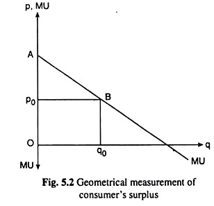
Now assume that q is a continuous variable and it is measured in infinitesimally small units, then the MU curve would be like the curve shown in Fig. 5.2. In this figure the consumer’s surplus would be obtained as an area. For example, if the price of the good is given to be p₀ in Fig. 5.2, the consumer would be in equilibrium if he buys the quantity q₀, for then he would be able to equate MU to p.

Since, at any quantity purchased, TU = ƩMU, here at q = q₀, TU would be equal to □OABq₀, which is the area under the MU curve at q = q₀, and the consumer’s total expenditure, on the other hand; would be p x q which at (p₀, q₀), would be equal to □Op₀Bq₀. Therefore, at p = p₀, the consumer’s surplus would be obtained to be □OABq₀ − □Op₀Bq₀ = □Ap₀B.

2. Consumer Equilibrium in the More-than-One Commodity Case:

Consumer equilibrium is discussed in the single commodity case. But in the real world, the consumer purchases a large number of commodities. So let’s discuss now the more- than-one commodity case. The simplest such case is where the consumer buys only two goods.

The Assumptions:

To conduct this analysis make the following assumptions:

(i) The consumer purchases only two goods, X and Y.

(ii) The prices of these goods are given in the market. They are p_x and p_Y. The consumer cannot change or influence these prices. He can only decide how much to buy of the goods at these given prices.

(iii) The consumer’s income to be spent on these goods is given and constant.

(iv) The consumer is a rational human being, and, as such, his goal here is to maximise the (cardinal) amount of utility from his purchase (and consumption) of the goods subject to his income constraint.

The rational consumer, in order to maximise utility from his purchase, should distribute his income over the purchase of the two goods in such a way that the marginal utility (MU) of money spent on each good may become the same.

In order to elaborate the idea, first note that the MU of money spent on any good, say X, is defined as the increment in total utility obtained from the consumption of X when an additional or the marginal unit of money is spent on X.

It follows from this definition that MU of money spent on X (MU^X_m) is equal to MU_X/p_X. This is very easy to understand. If the consumer spends an additional p_x amount of money on good X, he would be able to consume an additional unit of X, which would give him an additional utility of MU_X.

Therefore, for each additional or marginal unit of money spent on X, the consumer would obtain an additional utility of MU_Y/p_Y. That is, the MU of money spent on X is MU_X/p_X. Similarly, the MU of money spent on good Y would be equal to MU_Y/p_Y.

Now note that as the consumer spends more (less) money on X, he purchases and uses more (less) of X, and because of LDMU, MU_X falls (rises) leading to a fall (rise) in MU_X/p_X.

(p_x = constant)

Similarly, as the consumer spends more (less) money on Y, MU_Y/p_Y falls (rises). It is important to note here that the MU of money spent on any good would be diminishing (increasing) as the consumer spends more (less) money on the good, because of the LDMU.

Now, if the consumer randomly distributes his income over the purchase of the two goods and if he finds that MU of money to be spent on X is larger than MU of money to be spent on Y, then that is not a rational distribution.

For if he now reduces the money to be spent on Y and increases the money to be spent on X, then he would gain more than what he loses in terms of utility, i.e., his total utility would increase.

For example, if MU_X/p_X = 50 and MU_Y/p_Y = 30, then if the consumer spends Re 1 less on Y and Re 1 more on X, he would gain Rs 50 of utility from X and lose Rs 30 of utility from Y, thereby increasing his TU from spending his income by Rs 20.

He would, therefore, go on reducing the amount of money to be spent on Y and increasing the amount of money to be spent on X.

As a result MU_X, and so MU_X/p_X, would be falling and MU_Y, and so MU_Y/p_Y, would be rising, and at some particular distribution of the money, then:

MU_X/p_X= MU_Y/p_Y. At this particular distribution of his income, he would be able to obtain the maximum utility subject to his income because no further rise in TU is possible by a reallocation of his income.

Therefore, in this two-commodity case, the condition for consumer equilibrium is:

MU_X/p_X= MU_Y/p_Y                                                                                        (5.2)

i.e., the MU of money spent on each good should be the same, or, the MU of each good should be proportional to its price, as is seen in (5.2).

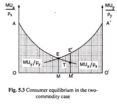
It is illustrated that the consumer equilibrium condition in the two-commodity case graphi­cally also, with the help of Fig. 5.3.

In Fig. 5.3, the fixed amount of money with the consumer to be spent on X and Y is represented by OO’. Along the vertical axis with origin O, measure the MU of money spent origin O’ measure MU of money spent on X (MU_X/p_X) and along the vertical axis with origin O’ measure MU of money spent on Y(MU_Y/p_Y).

The money spent by the consumer on good X is measured (rightward) along the axis OO’ and the money spent on good Y is measured (leftward) along the axis O’O. The MU_X/p_X curve gives us the MU of money spent on good X at any amount of money to be spent on X. This curve is sloping downward towards right because, as the money spent on X increases, MU_X/p_X, falls (because of LDMU_X).

Similarly, the curve MU_Y/p_Y gives us the MU of money spent on Y. This curve also shows that, as money spent on Y increases, MU_Y/p_Y falls (because of LDMU_Y). That is why this curve would slope down­wards towards left as the money spent on Y increases (from right to left) along the axis O’O.

Now, at the point of intersection E of the MU_X/p_X and MU_Y/p_Y curves, the consumer spends OM amount of money on X and O’M amount of money on Y. At this distribution of his income MU_X/p_X and MU_Y/p_Y become equal, both being equal to EM, and so here the consumer is able to maximise the amount of utility, or here he is in equilibrium.

The utility obtained at this distribution is the maximum subject to his income constraint, see, in Fig. 5.3, that at any other distribution of his income on the two goods, he would obtain a smaller amount of utility.

In Fig. 5.3, when the consumer spends OM of money on good X, he derives a utility equal to DOAEM. This is because TU of money spent on X = ∑MU of money spent on X. Similarly, when he spends O’M of money on Y the utility derived by him is equal to □ O’A’EM. There­fore, the total utility derived by him from spending all his income on X and Y is equal to □ OAEA’O’.

Now see what would be the amount of utility if he distributes his money in a different way. Suppose, for example, the consumer selects the distribution as repre­sented by any point other than M, say the point M’, on the 00′-axis. That is, he decides to spend OM’ of money on X and O’M’ of money on Y. Note that at this distribution MU_X/p_X ≠ MU_Y/p_Y; MU_X/p_X = TM’ < MU_Y/p_Y = E’M’.

This happens because the consumer now spends more money on X leading to a fall in MU_X and less money on Y leading to rise in MU_Y.

So at the distribution given by point M’, the condition for consumer equilibrium is not satisfied. At M’, the consumer derives the utility equal to DOATM’ from spending OM’ of money on good X and he derives utility equal to □O’A’E’M’ from spending O’M’ of income on Y.

Therefore, the total amount of utility derived by him from spending all his income would be □OATM’ + □O’A’E’M’ = □ OATE’A’O’. This area is less than the earlier TU area by □ETE’.

Hence it is proved that while distributing his money on the two goods, if the consumer ensures the equality of MU_X/p_X and MU_Y/p_Y, then he would be able to achieve utility maximisation. As also seen that at any distribution other than that given by point M, MU_X/p_X would not be equal to MU_Y/p_Y, and utility would not be maximum.

3. From Consumer Equilibrium to Law of Demand in the Two-Commodity Case:

For the two-good case, the condition for consumer equilibrium is:

MU_X/p_X ≠ MU_Y/p_Y                                                                         [eq.(5.2)]

If now p_x falls, other things, viz., p_Y and consumer’s money income, remaining the same, MU of money spent on X (MU_X/p_X) at the initial quantity purchased of good X rises, MU of money spent on (MU_Y/p_Y) remaining constant, i.e., now would become greater than MU_Y/p_Y.

As a result, the consumer would be reducing his expenditure on Y and increasing his expenditure on X, thereby increasing his demand for X, and moving towards a new equilib­rium. In other words, as p_x falls, ceteris paribus, demand for X rises.

Similarly, if p_x rises, ceteris paribus, his demand for X would fall. Therefore, in the two-good case also, deduce the law of demand from the Marshallian introspective cardinal utility analysis.