Perfect Substitutes:
In some cases of consumption, a two-good (X and Y) consumer may prefer to substitute one of the goods, say, X, for the other good Y at a constant rate, to keep his level of utility constant, i.e., MRSX,Y = constant. For example, he may always want to substitute one red pencil for one blue pencil, to keep him-self on the same indifference curve (IC).
In this case, naturally, his level of utility would depend on the total number of pencils, not on how many of the pencils are red and how many of them are blue, provided the consumer has no fascination for any particular colour.
Therefore, his utility function may be written as:
U = x + y (6.93)
ADVERTISEMENTS:
where x and y are, respectively, the number of red and blue pencils.
However, (6.93) is not the only utility function it could be used to represent the consumer’s preference pattern under discussion. For, any positive monotonic transformation of the function may serve our purpose. Therefore, it could also use the square of the total number of pencils to determine his utility level.
That is, his utility function may also be:
V (x, y) = (x + y)2 = x2 + 2xy + y2 (6.94)
ADVERTISEMENTS:
It is obvious that (6.94) is a positive monotonic transformation of (6.93). Now see how the utility function would look like if the consumer substitutes good X for good Y at a rate other than one-to-one. Suppose, for example, that the consumer substitutes 1 unit of good X for 2 units of good Y.
In this case, the MRSX, y is equal to 2, i .e., the slope of the IC = −2, and, therefore, the equation of the IC would be U0 = 2x + y, and, therefore, the utility function would be
U (x, y) = 2x + y (6.95)
In general, preferences for perfect substitutes can be represented by a utility function of the form:
ADVERTISEMENTS:
U (x,y) = ax + by
Here a and b are positive numbers, the MRSx.y = a/b = constant, the slope of an IC would be – a/b = constant. Since MRSx.y = a/b, the value of 1 marginal unit of good X to the consumer is equal to a/b unit of good Y, or, the value of ’b’ unit of good X, on the margin, is equal to ‘a’ unit of good y.
(A) Implications of Constant Marginal Rate of Substitution for the Indifference Curves and Consumer Equilibrium:
Suppose, the consumer uses only two goods X and Y, both of which are of more-is-better (MIB) type. One of the standard assumptions of the indifference curve (IC) theory is that of diminishing marginal rate of substitution of good X for good Y (MRSX,Y) as the consumer substitutes X for Y.
The axioms of MIB and of diminishing MRS give rise to two of the standard properties of the ICs—the ICs are negatively sloped and convex to the origin. Therefore, if the MRSX,Y is not diminishing, if it is constant or increasing, the ICs would be negatively sloped, but not convex to the origin.
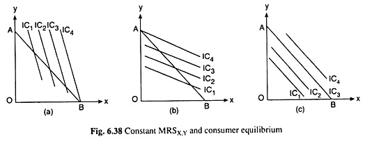
Let’s first discuss the implications of constant MRS. By definition, MRSX,Y at any point on an IC is equal to the numerical slope of the IC at that point. Therefore, constancy of MRSX,Y would imply that the consumer’s ICs would be negatively sloped straight lines, as shown in parts (a), (b) and (c) of Fig. 6.37.
Now let’s discuss the implications of negatively sloped straight line ICs for consumer equilibrium. If the ICs are convex to the origin, the equilibrium of the consumer would be obtained at the point of tangency between his budget line and one of his ICs.
But when the ICs are negatively sloped straight lines, none of them can have a point of tangency with a linear budget line. So, here, there is no point-of-tangency equilibrium. Instead, here there are three different cases.
In the first case, if the ICs are negatively sloped straight lines and each of them is steeper than the budget line, as shown in Fig. 6.38(a), then as the consumer moves downward towards right along his budget line, he would be reaching higher and higher ICs.
ADVERTISEMENTS:
Finally, at the corner point B of the budget line with the x-axis, the consumer would be in equilibrium because, at this point on the budget line, he is on the highest possible IC, viz., IC4.
The equilibrium at a corner point is called a corner solution or a boundary solution. Here at the corner solution given by point B, the consumer would buy only good X and no Y, i.e., he would spend all his money on X. Obviously, in this case, the consumer would have a unique equilibrium solution.
The economic interpretation of why the consumer would be in equilibrium at the corner point B, is this. Here, at any point on the budget line, the numerical slope of an IC, or, the MRSX Y, or, the significance of the marginal unit of X in terms of Y, is greater than the numerical slope of the budget line, or, the market price of X in terms of Y.
On the other hand, the significance of the marginal unit of good Y in terms of X would be smaller than the market price of Y in terms of X. Therefore, the utility-maximising consumer would monotonically go on increasing his purchase of good X and decreasing his purchase of good Y along his budget line till he hits the extreme at point B.
ADVERTISEMENTS:
In the second case, which is just the opposite of the first case, if the negatively sloped straight line ICs are flatter than the budget line, as has been shown in Fig. 6.38(b), then as the consumer moves upward towards left along his budget line, he would be reaching higher and higher ICs, and finally at the corner point, A, of the budget line with the y-axis, the consumer would be in-equilibrium, since at this point, he would be on the highest possible IC, viz., IC4.
Therefore, in this case also, it would have a unique corner solution. At the corner point A, the consumer would buy only Y (OA of Y) and no X.
The economic interpretation of why the consumer would be in equilibrium at the point A is that, here, since the ICs are flatter than the budget line, the significance of the marginal unit of X in terms of Y at any point on the budget line, is smaller than the market price of X in terms of Y, and therefore, the significance of the marginal unit of Y in terms of X is greater than the market price of Y in terms of X.
Therefore, the consumer here would go on increasing his purchase of Y and decreasing his purchase of X till he hits the point A.
ADVERTISEMENTS:
Finally, in the third case, if the negatively sloped straight line ICs are parallel to the budget line, then one of the ICs would coincide with the budget line, for example, IC3 in Fig. 6.38(c). This IC (i.e., IC3) is the highest curve that the consumer can reach subject to his budget constraint. Any point on this IC, which is also a point on the budget line, may be taken to be the consumer’s equilibrium point.
Therefore, here, the consumer has not a unique equilibrium solution—he may have a large number of equilibrium points. Also, all the equilibrium points (on the budget line) barring the two corner points, are non-corner solutions. At these points the consumer would buy a combination of both the goods.
The economic interpretation of this third case may be given like this. Here, since the numerical slope of the IC is equal to that of the budget line, and so, the marginal significance of X (or Y) in terms of Y (or X) is equal to the market price of X (or Y) in terms of Y (or X) at any point on the IC that coincides with the budget line, the consumer is equally satisfied with all these points.
So any point on this IC subject to his budget, may be his equilibrium point.
Thus, it is seen in the analysis that if the MRS is constant, the consumer’s ICs would be negatively sloped straight lines. So far his equilibrium is concerned, here three distinct cases are obtained.
ADVERTISEMENTS:
In the first two cases, the consumer would have corner equilibrium solutions—he would buy only X in the first case and only Y in the second case. In the third case, the consumer would have no unique solution. He may have a large number of solutions— corner or non-corner.
(B) The Nature of Consumer Equilibrium and the Price, Income and Substitution Effects:
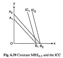
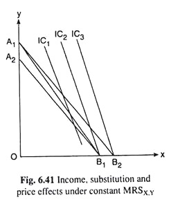
In the case of negatively sloped straight line ICs, if the ICs are steeper than the budget line, equilibrium of the consumer will be obtained at the corner point of the budget line with the horizontal axis. At this point, the consumer will buy only good X and no Y. For example, in Fig. 6.39, with the budget line A1B1, the consumer equilibrium has been obtained at the point B1 the consumer buying OB1 of X and zero of Y.
If now the consumer’s money income rises, prices of the goods remaining the same, his budget line would have a parallel rightward shift from A1B1 to A2B2 and his equilibrium corner solution would move from point B1 to point B2.
As the consumer’s money income, and also his real income, rises he moves from the lower IC, IC1, to the higher IC, IC2. Of course, he spends all his money on X buying OB2 of X and nothing of Y.
Here the consumer’s ICC can be obtained by joining the point of origin, O, and the points B1, B2, etc. Obviously, his ICC would be the horizontal axis or the x-axis itself. Also, here, when his money income (M) is zero, he buys zero of both the goods at the point of origin O.
ADVERTISEMENTS:
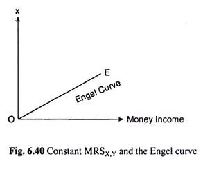
As M rises, his purchase of X rises proportionately, since he spends all his money (M) on X and the price of X remains constant. That is why his Engel Curve would be an upward sloping straight line through the origin, the level of this curve depending on the price of X—the level being higher, the lower the price of X.
Now try to explain the price effect (PE) in the constant MRS case, and the break-up of this effect into a substitution effect (SE) and an income effect (IE), with the help of Fig. 6.41. Let us suppose that, initially, the consumer’s budget line is A1B1 and his equilibrium occurs at the point B1—he buys OB1 of X and zero of Y on IC2.
Now suppose that the price of X falls, ceteris paribus, and his budget line rotates from A1B1 to A1B2. His equilibrium point now would be the corner point B2. He now moves to a higher IC, viz., IC3, as his real income has increased, and he now purchases B1B2 more of X because of the PE, and continue to buy zero of Y. Here the price-effect is the movement in his equilibrium point from B1 to B2.
In order to know the substitution effect portion of the price effect, let us now apply the Slutsky compensating variation in income by reducing his money income by B1B2 in terms of X or A1A2 in terms of Y, so that his budget line may have a parallel leftward shift from A1B2 to A2B1, and he may be able to buy the initial combination B1. However, when his budget line is A2B1 he would be in equilibrium also at the point B1.
ADVERTISEMENTS:
Compare his initial equilibrium point B1 with his new equilibrium point B1 it is found that the substitution effect upon his purchase plan is zero. This is because no substitution is possible here, as the consumer always buys zero of Y and spends all his income on X (whatever may be his budget line).
Now give him back the money income that is taken away from him, his budget line would have a parallel shift from A2B1 to A1B2 and his equilibrium point would move from B1 to B2—this movement represents the income effect.
The same movement represents the price effect. Therefore, here income effect and price effect would be identical. This is obvious, as there is no substitution effect.
It may be noted here that, in the case under consideration, both the income-consumption and price-consumption curves would be the horizontal (x-) axis itself, since as a result of both income and price changes, the consumer’s equilibrium point moves along the x-axis.
(C) Price-Demand Relations in the Case of Constant MRS:
The following demand relations in the case of constant MRS are obtained:
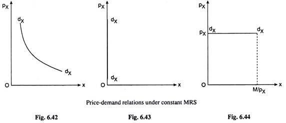
(i) If the budget line is flatter than the indifference curves (ICs), the consumer would spend all his money income (M) on good X, i.e., his demand for good X would be
ADVERTISEMENTS:
x = M/px v (6.97)
Since M is constant, eqn. (6.97) gives that the demand curve for good X (dxdx) in this case would be a rectangular hyperbola as shown in Fig. 6.42.
(ii) If the ICs are flatter than the budget line, the consumer would spend all his money on Y and he would demand zero of good X at any price, i.e.,
x = 0 (6.98)
Equation (6.98) gives the demand curve (dxdx) for good X in this case would be the px-axis itself (Fig. 6.43).
(iii) If the slope of the budget line is the same as that of the ICs, then one of the ICs would coincide with the budget line. In this case, any point on the budget line may be the equilibrium point of the consumer, so that the consumer’s demand for good X may be any quantity between zero and M/px at the given px, (Fig. 6.44) i.e., we would have
X = any quantity between 0 ans M/pX, i.e., 0 ≤ x ≤ M/pX …….(6.99)
Equation (6.99) gives the demand curve (dxdx) in this case would be the curve as given in Fig. 6.44 ― it would be horizontal straight line at the level of px subject to x ≤ M/pX
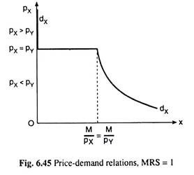
An interesting special case of price-demand relation in the constant MRS preference pattern, would be obtained when the consumer’s MRSX,Y = 1, i.e., when the numerical slope of his ICs is equal to 1.
Here, three cases are obtained:
(a) For px > pY, the budget line would be steeper than the ICs, and the equilibrium solution would be obtained at the upper corner of the budget line, i.e., the consumer would buy a zero quantity of good X, i.e., the vertical (px) axis of Fig. 6.45 would be the consumer’s demand curve for good X.
(b) For px = Py the budget line would be parallel to the ICs — the numerical slope of both of them would be equal to 1. Therefore, at any px, demand for X would be anything between zero and M/pX. So, in this case, the demand curve for good X would be a horizontal straight line at the level of px over 0 ≤ x ≤ M/pX = M/pY (pX = pY).
(c) For px < py, the budget line would be flatter than the indifference curves, its numerical slope being less than 1. Here at any px, the consumer’s demand for X would be M/pX, i.e.,
x = M/pX .
or, px.x = M = constant. In this case, the consumer’s demand curve for X would be a rectangular hyperbola.
It is obtained, therefore, that under MRSX,Y = 1, the consumer’s demand curve for good X would be like dxdx, in Fig. 6.45—first, the curve would have a vertical segment for pX > PY, then it would have a horizontal segment for px = pY, and lastly, the curve would have a rectangular hyperbola segment for pX < pY.
The price-demand relations between the demand for good Y and its price can be obtained in just the same way as obtained the in relations of the case of good X.
(D) The Income-Demand Relations when the MRSX,Y is Constant:
From,
x = M/px [eqn.(6.97)]
it is obtained that px remaining constant, as M (money income) increases, x (demand for good X) also increase and x is proportional to M, i.e., if M increases t times (where t is a positive real number), x also increases t times.
It may be noted here that equation (6.97) is the demand curve for good X if M remains unchanged—it would then be a relation between px and x; and the same equation is the Engel curve for good X if px remains unchanged—it would then be a relation between M and x.
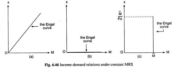
As is evident from equation (6.97), the Engel curve, which is the relation between M and x, is a straight line, and measure M along the horizontal axis and x along the vertical axis, then the slope of the Engel curve would be equal to 1/px = positive [Fig. 6.46(a)],
When the ICs are flatter than the budget line, and equilibrium is a corner or boundary solution on the y-axis, the consumer’s demand for good X would be zero whatever may be his income. So in this case income-demand relation is
x = 0 [(6.98)]
at each M (income), which is also the equation of the Engel curve for good X. Measure x along the vertical axis and M along the horizontal axis, then the Engel curve in this case would be the horizontal (M) axis itself [Fig. 6.46(b)].
Lastly, when the ICs are parallel to the budget line, the consumer would be in equilibrium at any point on the budget line or on the indifference curve that happens to coincide with the budget line.
In this case, at any given M, the consumer’s demand for good X may assume any value between zero and M/px. Therefore, in this case, the Engel curve [shown in Fig. 6.46(c)] would be a vertical straight line at the given M = M̅ over the range 0 ≤ x ≤ M̅/px.
The Horizontal or Vertical Straight Line Indifference Curves:
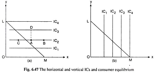
Of the two goods that the consumer purchases, if one is “more-is-better” and the other is neither “more-is-better” (MIB), nor “more-is-worse” (MIW), then he would have his ICs to be horizontal or vertical straight lines. For example, suppose, good Y measured along the vertical axis is an MIB and good X measured along the horizontal axis is neither an MIB nor an MIW, i.e., MUX = 0 and MUY > 0.
In this case, more of good Y will give the consumer a higher level of satisfaction, but more or less of good X will make no difference to his level of satisfaction. Therefore, here the ICs of the consumer will be horizontal straight lines like the ones shown in Fig. 6.47(a).
If the consumer moves along a particular IC, from one point to another, e.g., if he moves from any point A to any other point B, or, C along any particular IC, say, IC2, then he would have more or less of good X which would not change his level of satisfaction, since MUX = 0.
On the other hand, as he moves from A to B, or, to C, he would have no change in the amount of Y. Therefore, although MUY > 0, his level of satisfaction would remain constant at these points. That is, the consumer would be indifferent between the points A, B and C along IC2 which is, therefore, one of his ICs.
In Fig. 6.47(a), the consumer’s map is horizontal to ICs. In this indifference map, note, a higher IC represents a higher level of utility.
For example, if the consumer moves vertically from point A on IC2 to point D on a higher IC, viz., IC3, his level of satisfaction will rise because, at the point D, as compared with A, he would have a larger quantity of the MIB good, Y, along with the same amount of good X. (Of course, here even if there had been a change in the amount of X, it did not matter, since MUX = 0)
If the ICs are negatively sloped straight lines and are flatter than the consumer’s budget line, then his equilibrium solution would be a corner or boundary solution at the corner point of the budget line with the vertical axis.
Here also, the same thing happens. Since the ICs are flattest to the limit, being horizontal straight lines, the consumer’s equilibrium solution would be obtained at the corner point of the budget line with the vertical axis.
In Fig. 6.47(a), this point is point L where the budget line takes the consumer to the highest possible IC, viz., IC4. At this point, the consumer would buy only Y and no X. The economics of this decision lies in our assumptions of MUX = 0 and MUY > 0.
In a similar analysis, it is seen that if MUX > 0 and MUY = 0, then the consumer’s ICs will be vertical straight lines as shown in Fig. 6.47(b). In this case, of any two ICs, the one which is to the right of the other will represent a higher level of satisfaction. For example, the utility level of IC4 > the utility level of IC3 > the utility level of IC2 > the utility level of IC1.
This is because as the consumer moves horizontally from any point on one IC to another point on an IC to the right, he would have more of good X, the amount of good Y remaining the same. Since MUX > 0 and MUY = 0, he would reach a higher level of satisfaction in the process.
If the ICs are negatively sloped straight lines and steeper than the budget line, then the consumer’s equilibrium point would be the corner point of the budget line with the horizontal axis. In the case, since the vertical straight line ICs are steepest to the limit, the consumer’s equilibrium point would be the corner point M of the budget line with the horizontal axis.
At this point the consumer would be on the highest possible IC, viz., IC4, and he would purchase only good X and no Y. The economic interpretation of why he would purchase only X and no Y is given by the fact that here it is assumed MUX > 0 and MUY = 0.
Increasing Marginal Rate of Substitution:
A case may be observed like this: a two-good consumer likes to have more of both the goods, i.e., both the goods are MIBs to him, but he does not like to have both the goods at the same time, e.g., he may like to have both tea and biscuits but not both at the same time. In a case like this, obviously, the consumer’s optimal choice would have only one of the two goods and none of the other.
In order to arrive at the consumer’s equilibrium point in such a case, take note of the fact at the very beginning that here, if the two goods are X and Y, then by the nature of the problem, the consumer while moving along his indifference curve would want to forego one of the goods, say, Y, in order to have one more unit of the other good, X, at an increasing rate, i.e., here, the marginal rate of substitution of X for Y(MRSX,Y) would be increasing as the consumer goes on substituting X for Y. In other words, this is a case of increasing MRS as opposed to our usual assumption of diminishing MRS.
(A) Implications of Increasing MRS for the Indifference Curves and Consumer Equilibrium:
Let’s now examine the implications of increasing MRS for the indifference curve analysis. If the MRSX,V is increasing as the consumer substitutes good X for good Y, the ICs of the consumer would not be convex to the origin.
Since MRSX,Y at any point on an IC is equal to the numerical slope of the curve at that point, increasing MRSX Y implies that, as the consumer has more and more of X and less and less of Y, i.e., as he moves downwards along the IC, the numerical slope of the curve increases, i.e., the curve becomes steeper, which gives us that the ICs here would be concave to the origin.
Let’s now see what does this concavity imply for the equilibrium of the consumer. The point of tangency is the first-order condition (FOC) and the convexity to the origin of the ICs is the second order condition (SOC) for consumer equilibrium or utility- maximisation.
Therefore, if the FOC is satisfied at the point of tangency between the budget line and an IC, but there is concavity of the ICs, i.e., the SOC is not satisfied, then the point (of tangency) would not be the point of maximum utility, rather, it would be the point of minimum utility.
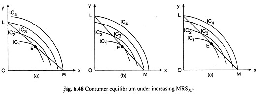
It may be seen in any part of Fig. 6.48. Here the point of tangency E on the budget line LM is not the utility-maximising point, for as the consumer moves along his budget line downward towards right or upward towards left of the point E, he moves on to higher and higher ICs.
Therefore, the point of tangency E on his budget line is not the utility-maximising point, rather, it is the utility-minimising point. The consumer cannot be in equilibrium at this point. So he would leave this point and proceed downward towards right or upward towards left along his budget line and moves on to higher and higher ICs.
Ultimately the consumer would reach point M on the x-axis, or, the point L on the y-axis. Now, he would have to compare the satisfaction levels at the points M and L. Here it is seen in Fig. 6.48(a) that, the point M lies on a higher IC, viz., IC4 than the point L which lies on IC3.
Therefore, in this figure, the consumer would ultimately be in equilibrium at the point M on IC4. Since the point M is a corner point of the budget line, here there is a corner solution. At the point M, the consumer would buy only good X (OM of X) and no Y. However, the equilibrium here is a unique equilibrium.
Again, in Fig. 6.48(b), the point L lies on a higher IC, viz., IC4 than the point M which lies on IC3. Therefore, in this figure, the consumer would be in equilibrium at the corner point L on IC4. So, here also, there is a unique corner solution. At this corner, the consumer would buy only good Y (OL of Y) and no X.
Lastly, in Fig. 6.48(c), both the corner points, L and M on the budget line, lie on the same IC, viz., IC4. Therefore, in this case, the consumer is indifferent between the points L and M— both the points may be his equilibrium point since both lie on the highest possible IC subject to his budget.
If he decides to stay at point M, he will buy only X and if he chooses to stay at the point L, he will buy only Y. Therefore, in this third case, the consumer will have a corner solution, but the solution is not unique.
It can now attempt at an economic interpretation of the decision-making behaviour of the consumer in this case. If the MRS is increasing, his ICs would be concave to the origin and he would have a corner equilibrium solution.
Since the ICs are concave to the origin, the consumer, when he leaves the point of tangency E and moves downward towards right along his budget line, will find that the ICs are steeper than budget line, i.e., the marginal significance of X in terms of Y is greater than the market price of X in terms of Y. Therefore, he would want to purchase more of X and move still downward towards right.
The process would go on till the consumer reaches the corner point M where he would spend all his money on X and buy the maximum possible amount of X (OM) and, of course, zero of Y.
Similarly, if the consumer moves upward towards left along his budget line leaving the point E, he would come across the ICs that are flatter than the budget line, i.e. the marginal significance of Y in terms of X is greater than the market price of Y in terms of X.
So now the consumer would want to purchase more of Y and he would be moving upward towards left along his budget line till he reaches the corner point L, where he would spend all his money on Y and buy the maximum possible amount of Y (OL) and zero of X.
Standard Indifference Curves Leading to Unusual Results:
Sometimes it may happen that the indifference curves possess all their ‘standard’ properties, yet, they do not lead to tangency or interior equilibrium solution.
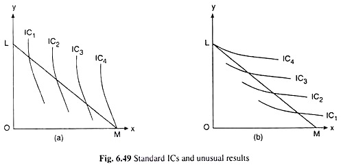
If the negatively sloped, convex-to-the-origin and non-intersecting ICs based on all the standard axioms and assumptions of preferences, are steeper or flatter throughout their lengths than the budget line, the equilibrium solution would be obtained to be a corner solution, i.e., the consumer in this case would buy only one of the goods.
The case be illustrated with the help of figures 6.49(a) and (b). In Fig. 6.49(a), the ICs are steeper than the budget line. Here at any point on the budget line, the marginal significance of good X in terms of good Y is greater than the market price of X in terms of Y, and the marginal significance of Y in terms of X is smaller than the market price of Y in terms of X.
Therefore, the consumer would go on increasing his purchase of X and decreasing that of Y, i.e., he would be moving downward towards right along his budget line till he hits the corner M of the budget line. At the point M, he would buy good X only and spend nothing on good Y.
On the other hand, in Fig. 6.49(b), the ICs are flatter than the budget line. Therefore, here, at any point on the budget line, the marginal significance of good X in terms of good Y would be smaller than the market price of X in terms of Y, and the marginal significance of Y in terms of X would-be larger than the market price of Y in terms of X.
So, now, the consumer would go on increasing his purchase of Y and decreasing that of X, i.e., he would be moving upward towards left along his budget line till he reaches the corner L. At the point L, he would buy only good Y and spend nothing on good X.
The Positively Indifference Curves:
Of the two goods (say X and Y) that the consumer purchases, if one is “more-is-better” (MIB) with MU > 0 and the other is “more is worse” (MIW) with MU < 0, then the ICs of the consumer would be positively sloped. For example, suppose that good X is an MIB with MUX > 0 and good Y is an MIW with MUY < 0.
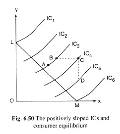
Now, of the two points, A and B, on any IC, say, IC3 in Fig. 6.50, if the consumer has more of X at B, then he should also have more of Y at B, in order to be indifferent between the two points. For, improvement in his level of satisfaction made possible by more of X should be duly cancelled by the deterioration of an equal extent in his level of satisfaction by way of an increase in his consumption of the MIW good, Y.
Therefore, the IC in this case between an MIB good and an MIW good would be positively sloped. The indifference map of a consumer consisting of positively sloped ICs has been given in Fig. 6.50. Now note that in Fig. 6.50, an IC farther from the y-axis would represent a higher level of satisfaction if good X is an MIB and good Y is an MIW.
For, if the consumer moves horizontally from the point B on IC3 to the point C on IC4, then at the latter point, he would have more of the MIB good, X along with an unchanged quantity of the MIW good Y. That is, here IC4 would represent a higher level of satisfaction than IC3.
On the other hand, if X is an MIW good and Y is an MIB good, then an IC farther from the x-axis would represent a higher level of satisfaction. For, now if the consumer moves, say, from the point D on IC5 to the point C on IC4, then at IC4 he would have more of the MIB good Y, along with the same quantity of the MIW good, X, i.e., here IC4 would represent a higher level of satisfaction than IC5.
That the IC between an MIB (with MU > 0) and an MIW (with MU < 0) would be positively sloped, can be established easily in terms of mathematics.
The slope of an IC is:
The Equilibrium Solution:
It is evident from Fig. 6.50 that the equilibrium solution in the case of positively sloped ICs would be a corner solution. If MUX > 0 and MUY < 0, i.e., if an IC farther from the y-axis represents a higher level of satisfaction, then equilibrium would occur at the corner point M on the budget line with the x-axis. The point M takes the consumer on to the curve IC6 which is the farthest from the y-axis subject to his budget.
At this point, the consumer would buy only good X and no Y. This is simply because X is an MIB good here and Y is an MIW good. On the other hand, if MUX < 0 and MUY > 0, i.e., if an IC farther from the x-axis represents a higher level of satisfaction, then equilibrium would take place at the corner point L on the budget line with the y-axis.
The point L takes the consumer on to the curve IC1 which is farthest from the x-axis subject to his budget. At this point, the consumer would buy only good Y and no X. This is because here Y is an MIB good and X is an MIW good.
The Income, Substitution and Price Effects for the Preference Patterns with a Corner Solution:
If the equilibrium solution is obtained at the corner of the budget line with the horizontal axis along which the quantity of good X is measured, then the following will be obtained:
(i) The substitution effect of a change in the price of X upon its purchase is zero.
(ii) Therefore, the price effect of this price change is identical with its income effect.
(iii) That is why both the income-consumption and price-consumption curves would be identical and would coincide with the horizontal axis.
The substitution is not obtained individually, income and price effects, and the ICC and the PCC is not derived because all these characteristics would be the same in these cases and mentioned in (i), (ii) and (iii) above.
The Negatively Sloped ICs with the Higher Curve Representing a Lower Level of Utility:
If both the goods (say, X and Y) that the consumer purchases are more-is-worse (MIW), then the consumer’s ICs would be negatively sloped with the higher curve (i.e. the one farther from the origin) representing a lower level of satisfaction.
In this case, the ICs would be negatively sloped because if the consumer moves from one point to another on the same curve getting a larger quantity of good X, and therefore, obtaining a lower level of satisfaction at the second point, then the quantity of good Y at this point must be appropriately smaller so that his level of satisfaction might increase to the initial level and he might be indifferent between the two points.
The negative slope of the ICs can be easily established if MUX < 0 and MUY < 0 in eq. (6.8). Also, in this case, a higher IC would represent a lower level of satisfaction. This is because, as the consumer moves horizontally or vertically from a lower IC to a higher IC, he would obtain more of the MIW good, X or Y, the amount of the other MIW good, Y or X, remaining unchanged.
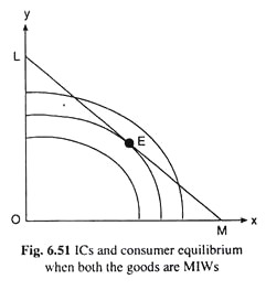
Now, assuming that as the consumer gets more of an MIW good, its negative utility on the margin increases (from, say, -2 to -3), then the MRSX,Y in this case where both the goods are MIWs, would increase as the consumer substitutes X for Y, i.e., his ICs here would be concave to the origin. Therefore, his indifference map consisting of these ICs would be like the one shown in Fig. 6.51.
The Equilibrium Solution:
If the consumer is subject to no constraint, then the maximum amount of utility that he would be willing to obtain from the two goods, is zero, because, here both the goods give him negative utility. Therefore, and so the equilibrium point of the consumer here would be the point of origin (x = 0, y = 0) in Fig. 6.51. Since both the goods give him a negative utility, he would prefer not to buy the goods.
On the other hand, if, theoretically, he is constrained to spend a certain sum of money on the two goods at given prices, he would have a budget line like LM in Fig. 6.51. Now, if the consumer’s indifference map is the one given in Fig. 6.51, then his equilibrium point would be the point of tangency E between the curve IC2 and his budget line.
Since the ICs here are concave to the origin, the point of tangency E takes the consumer to the lowest possible IC subject to his budget, i.e., to the highest possible level of utility, for here a lower IC represents a higher level of utility.
It may be noted here that the highest possible level of utility here would be negative with minimum absolute value, since the MUs for both the goods are negative. It may also be noted here that although the ICs here are concave to the origin, the equilibrium solution obtained here is not a corner solution—it is an interior solution.
Implications for the Shape of the Indifference Curves and the Equilibrium of the Consumer if the Marginal Utility of the Goods becomes Negative Eventually:
One of the standard assumptions of the indifference curve theory is that both the goods, say, X and Y, that the consumer uses are of more-is-better (MIB) type, i.e., the MUs of both the goods are positive. On the basis of this assumption, the standard properties of the ICs is obtained, viz., the ICs are negatively sloped curves.
Now, if this assumption is restricted to one where it is said that each good is an MIB for the consumer up to a certain quantity and then it would have negative MU for him, i.e., the good would become a more-is-worse (MIW) good, then the standard IC analysis would change in important ways. In order to proceed further, remember certain points.
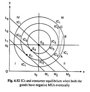
Refer to Fig. 6.52. Suppose that good X is an MIB for the consumer up to the quantity x0 and for x > x0, good X becomes an MIW. Similarly, good Y is an MIB for the consumer up to y = y0 and for y > y0, Y becomes an MIW.
In Fig. 6.52, the commodity space has been divided into four quadrants with the help of the vertical and the horizontal lines drawn at x = x0 and y = y0, respectively.
It follows from the assumptions:
(i) In quadrant I, both the goods are MIBs. So, the ICs going through the points in this quadrant would be negatively sloped, the higher IC representing a higher level of utility,
(ii) In quadrant II, one of the goods, X, becomes an MIW, although Y is an MIB.
Therefore, the portion of an IC passing through the points in this quadrant would be positively sloped, the higher (farther from the x-axis) IC here representing a higher level of utility,
(iii) In quadrant III, both the goods are MIWs. Therefore, the ICs passing through the points in this quadrant would be negatively sloped, but a higher IC here would represent a lower level of utility,
(iv) In quadrant IV, one of the goods, Y, is an MIW, but X is an MIB. So, here also, like quadrant II, the ICs would be positively sloped, but a higher IC (one farther from the x-axis) would represent a lower level of utility.
It follows from above that ICs under the given assumptions would be circular or elliptical, somewhere convex and somewhere concave, depending on the preference-indifference pattern of the consumer. Some such ICs have been given in Fig. 6.52.
Now go into the implications for the equilibrium of the consumer if his ICs are like those given in Fig. 6.52. Let’s first make it clear that if looking at IC in Fig. 6.52 in its totality, it is found that all its segments except that lying in the first quadrant are to be rejected prima facie by the utility-maximising consumer.
The reasons may be given in this way. Along the segment of an IC in the second quadrant, as the consumer moves upward towards right, he uses more of both the goods, but his utility remains the same. This follows from the fact that one of the goods, X, is MIW here. But this cannot be accepted by the consumer if he pays positive prices for the goods, which, is assumed, he does.
Again, as compared to the points on the segment of an IC in quadrant II, there are points on the quadrant III portion of the same IC that contain more of both the goods (compare the points A and B on IC1) or more of one good and the same quantity of the other (compare the points A and C on IC1). This follows from the fact that both the goods are MIWs in the third quadrant.
That is why the quadrant III segment of an IC becomes irrelevant for the consumer’s consideration. Lastly, as the consumer moves upward towards right along the positively sloped quadrant IV segment of an IC, he uses more of both the goods, but his level of utility remains unchanged.
This follows from the fact that one of the goods, Y, is MIW here. Therefore, the consumer would keep this segment of an IC out of his consideration.
However, the consumer cannot prima facie reject the points on an IC that lie in quadrant I. For, here, as he moves along an IC, his utility remains the same and it is not that he uses more of both the goods— rather as his use of one of the goods increases, that of the other good decreases. This follows from the fact that both the goods are MIBs in this quadrant, which is consistent with the assumption of utility maximisation.
From the analysis, it may be concluded that the ICs given in Fig. 6.52, only quadrant I is relevant for the consumer, and his equilibrium may be obtained only in this quadrant.
For example, if his budget line is L1M1, he would be in equilibrium at the point E1 on IC2, and if his budget increases, prices of the goods remaining constant, his budget line would have a parallel rightward shift to say L2M2, and now his equilibrium point would move from E1 to E2.
It may be noted here that as the ICs become higher in quadrant I representing a higher level of utility, the ‘circle’ of the IC would become smaller, and in the limit it would become a point. That point in Fig 6.52 is the point E3 which is the point of intersection of the horizontal and vertical lines at y = y0 and x = x0, respectively.
It may also be noted that under the circumstances given in Fig. 6.52, the consumer may go on increasing his expenditure till his budget line becomes L3M3.
With this budget line, he would be in equilibrium at the point E3 (x0, y0) which is the limiting point of both the goods being MIBs. Under the given circumstances, the consumer need not spend more money than that associated with the budget line L3M3, to maximise his level of satisfaction.
Implications for the ICs and Consumer Equilibrium if the Goods are to be used in a Fixed Proportion:
The standard assumption of the indifference curve analysis is that the two goods, say, X and Y, that the consumer uses can be substituted for one another subject to diminishing MRS. On the basis of this assumption, it is obtained that the ICs are convex to the origin.
If this assumption is replaced by the assumption that the goods, X and Y, are to be used in a fixed proportion, i.e., they are perfect complements to each other, no longer the ICs gets to be convex to the origin. Rather, it obtained to be L-shaped.
The point may now be explained with the help of Fig. 6.53, where it is assumed that the goods are always to be used in the ratio 1:1, which implies that the consumer has to use the combinations of the goods like A(1, 1), B(2, 2), C(3, 3), etc.
Since the goods are MIBs a combination of more of the goods gives the consumer a higher level of satisfaction, i.e., the IC on which the combination B (2, 2) lies is higher than that on which A (1, 1) lies.
Similarly, the IC on which C (3, 3) lies is higher than the one on which B(2, 2) lies, and so on. Again, since the goods are to be used in a fixed ratio, here 1:1, more of any good out of the ratio would add nothing to the consumer’s satisfaction level.
Thus, the consumer would be indifferent between the combinations (1, 1), (2, 1), (3, 1), . . ., (1, 2), (1, 3), (1, 4), . . and the formation shall be obtained when these points are joined, is an L-shaped IC, viz., IC1.
Similarly, the consumer would be indifferent between the combinations (2, 2), (3, 2), (4, 2), . . ., (2, 3), (2, 4), (2, 5), . . . and if these points are joined by a curve another L-shaped IC is is obtained like IC2; IC2 would be a higher curve and it would give the consumer a higher level of satisfaction, since B(2, 2) is preferable to A(l, 1).
Again, the consumer would be indifferent between the combinations (3, 3), (4, 3), (5, 3)…………… (3, 4), (3, 5), (3, 6),. .. and through these combinations shall get another L-shaped IC, viz., IC3; IC3 would be higher than IC2 and it would give the consumer a higher level of satisfaction than the latter, since C(3, 3) is preferable to B(2, 2).
Therefore it is seen that if the goods are to be used in a fixed ratio, then the ICs would be L-shaped—the horizontal arm of the L contains the combinations of the same quantity of Y and more and more of X, and the vertical arm of the L contains the same quantity of X and more and more of Y, and the meeting point of these two arms like the point A or B, etc. in Fig. 6.53 represents the combination where the quantities of the goods are in the required ratio (here 1:1).
Let’s now see the implications of the L-shaped ICs for the equilibrium of the consumer. Suppose, the consumer’s ICs are those given in Fig. 6.53, and his budget line is the line EF.
In this figure, the line OR joining the points A, B, C, etc. and the point of origin ‘O’ may be called the line of X-Y relationship—it gives what should be the value of Y for any particular value of X, and what should be the value of X for any particular value of Y, so that the required ratio is maintained.
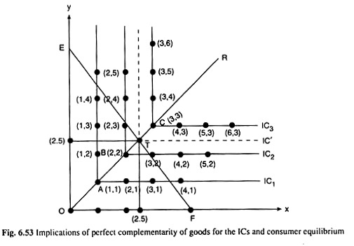
It is seen in Fig. 6.53 that the point T is a combination of 2.5 units of good X and 2.5 units of good Y. Since T is also a point on the X-Y relationship, it is ensured that the quantities of the goods are in the required ratio (here 1:1).
(A) Mathematical Expression for Perfect Complements:
Suppose, a two-good consumer is required to consume the two goods in a fixed ratio. For example, he has to use the left shoe and the right shoe in a 1 : 1 ratio.
So it is natural in this case that the level of utility is a function of the number of complete pairs of shoes, not of the total number of left and right shoes. Now, the number of complete pairs of shoes the consumer may have is the minimum of the number of right shoes, say, x and the number of left shoes, say, y.
Thus the utility function of perfect complements takes the form:
U (x, y) = min {x, y} (6.100)
Also, any monotonic transformation of (6.100) would also be a suitable utility function, representing the same preferences.
There may also be cases where the consumer has to use the goods in a ratio other than 1:1. Let’s see how to obtain the utility function in such a case. Suppose that the consumer uses 2 teaspoons of sugar with each cup of tea—the number of cups of tea being denoted by x and the number of teaspoons of sugar by y. Therefore, in this case, the number of
As usual, any monotonic transformation of (6.101) will also represent the same preferences.
So, here, to get rid of the fraction 1/2, shall apply a monotonic transformation by multiplying (6.101) by 2, and then the utility function can be obtained as
U (x, y) = min {2x, y} …(6.102)
In general, a utility function that describes the perfect complement preferences is given by
U (x, y) = min {ax, by} …(6.103)
where a and b are positive numbers and the goods X and Y are consumed in the ratio b : a.
(B) Demand Relations under Perfect Complementarity:
For a given money income, M, and for the given prices px and pY of the goods, the consumer’s budget constraint is
pxx + pyy = M …(6.104)
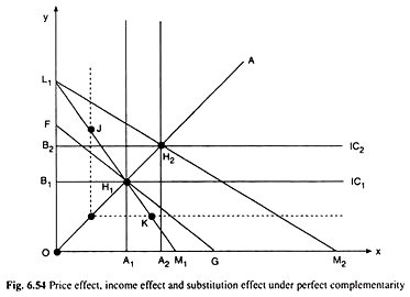
The consumer can purchase at any point on the budget line (6.104), e.g., the line L1M1 in Fig. 6.54. But the optimal choice will be obtained at the point H1 on L1M1 where the consumer is on the highest possible IC subject to his budget.
Now, under perfect complementarity, the consumer has to use the goods in a fixed ratio, say, m : n. Therefore, at the equilibrium choice like H1 we would have
Eqn (6.106) gives the demand function for good X under conditions of perfect complementarity—demand for X is a function of px, py and M. In the same way, the demand function for good Y would be obtained to be
It is seen from (6.106) and (6.107) that, since the goods X and Y are complements, increase in px and/or pY would cause a fall in the demand for each good. [... px and pY are in the denominator of the RHS expressions of (6.106) and (6.107). However, an increase in M would cause a rise in their demands (... M is in the numerator of the RHS expressions)].
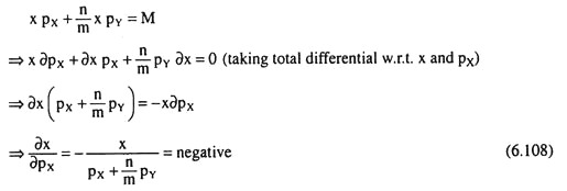
From (6.106), we have
Eqn. (6.108) gives the slope of the demand function for good X, which has been obtained to be negative. Similarly, the slope of the demand function (6.107)is obtained for good Y as
Therefore, as already obtained and now (6.108) and (6.109), also, gives that, under conditions of perfect complementarity, the demand for each good is inversely related to its price. It is also obtained in Fig. 6.54, that as the price of good X falls and the budget line rotates from L1M1 to L1M2, the consumer’s purchase of good X increases from OA1 to OA2.
(C) Income-Demand Relations:
If px and pY remain constant, then demand function (6.106) itself becomes the income-demand relation for good X, known as the Engel curve for good X. The slope of this curve is
Similarly, if px and pY remain constant, (6.107) becomes the income-demand relation for good Y or the Engel curve for good Y. The slope of this curve is
Under conditions of perfect complementarity, the Engel curve is obtained for each good as a positively sloped straight line from the origin, i.e., as income increases, demand for each good also increases in the same proportion. This is already noted by inspection of (6.106) and (6.107).
(D) Price Effect, Income Effect and Substitution Effect under Perfect Complementarity:
Let’s now discuss the nature of consumer equilibrium and the effects of changes in money income and relative prices of the goods, upon this equilibrium under conditions of perfect complementarity. In Fig. 6.54, a negatively sloped linear budget line of the consumer like L1M1 would ‘touch’ one of the L-shaped ICs at its corner point, and this IC is the highest one that the budget line can take the consumer to.
For example, the budget line L1M1 would ‘touch’ IC1 at its corner point H1 At any other point on this budget line, e.g., at J or K, the consumer is on a lower IC. So when the budget line is L1M1, the consumer is in equilibrium at the corner point H1 on IC1.
Suppose, initially, the budget line of the consumer is L1M1 and he is in equilibrium at the point H1 where he purchases OA1 of good X and OB, of Y. Again suppose, the price of X falls, ceteris paribus, and the budget line of the consumer rotates as a result, from L1M1 to L1M2.
The new budget line ‘touches’ IC2 at the point H2. So the new equilibrium point is H2. The consumer is now on a higher IC, since his real income has increased. By definition, the movement of the equilibrium point of the consumer from H1 to H2 is the price-effect movement. On account of the price effect, the consumer purchases A1A2 more of X and B1B2 more of Y.
In order to isolate the substitution effect portion of the price effect, now notionally reduce the money income of the consumer by the amount of “compensating variation” so that his budget line would now have a leftward parallel shift to FG and it would ‘touch’ IC2 at the point H2 . Under conditions of perfect complementarity, both the lines L1M1 and FG ‘touch’ IC1 at the same corner point H1.
So, in this case, the substitution effect (SE) movement of the consumer’s equilibrium point is from H1 to H2 i.e., here there is no SE movement and the SE upon both the goods is zero. This is what is expected because, under conditions of perfect complementarity, substitution between the goods is not possible.
In order to obtain the income effect (IE) portion of the price effect, now return the money to the consumer, which is taken away from him in order to know the SE. His money income now increases, prices remaining constant.
As a result, due to IE, there would be a parallel rightward shift in his budget line from FG to L1M2 and his equilibrium point will move from H1 to H2, which is the same as the PE movement, i.e., the IE movement in his equilibrium point is the same as the PE movement. This is again expected because in this case SE movement is absent.
Because of the IE, the consumer purchases A1A2 more of X and B1B2 more of Y. Thus, under perfect complementarity, income effect is the same as the price effect, since the substitution effect is zero.
One more point should be noted. Under conditions of perfect complementarity, the (income-consumption curve) ICC of the consumer is obtained by joining the equilibrium points like H1 H2, etc. lying on the fixed x-y ratio line OA, and the (price-consumption curve) PCC of the consumer for good X is also obtained by joining the points H1 H2 etc.
Therefore, here the PCC for good X is the same as the ICC—this is the line OA. Also, it can be seen in the same way that PCC for good Y is the same as the ICC which is also OA; so here PCC for good X and that for good Y, and ICC, all are the same line OA. All this is due to the fact that the substitution effect is zero under conditions of perfect complementarity.
Cobb-Douglas Preference:
If the utility function of a consumer is of the form:
U(x, y) = xαyβ ….(6.112)
then his preference pattern would be called Cobb-Douglas preference. The function (6.112) is known as the Cobb-Douglas function named after the economists Cobb and Douglas. In (6.112) α and β are positive numbers and they describe the preferences of the consumer.
Cobb-Douglas ICs are well-behaved negatively sloped and convex-to-the-origin ICs. A positive monotonic transformation of a utility function will represent exactly the same preferences, and the Cobb-Douglas utility function is no exception. Here a couple of examples can be examined for such transformation.
First, if the natural log of utility is taken in (6.112) we would have
The ICs for the utility (V) function (6.113) will look just like those for the function (6.112), since taking logarithm is a positive monotonic transformation.
In the second case, suppose let’s with the Cobb-Douglas form:
This means that it can always take a monotonic transformation of the Cobb-Douglas utility function that makes the sum of the exponents equal to 1.
The optimal choices for the utility function (6.112) are
where px and pY are the prices of goods X and Y, and M is the money income of the consumer. The Cobb-Douglas preferences have a convenient property. The fraction of his income that a Cobb-Douglas consumer spends on good X is px x. Substituting from demand function, we have
pxx/M = px/M. α/α +β. M/px = α/α +β = constant (6.117)
Similarly, the fraction of his income that the consumer spends on good Y is
py.y/M = β/α +β = constant (6.118)
It is evident from (6.117) and (6.118) that the Cobb-Douglas consumer always spends a fixed fraction of his income on each good. The size of the fraction is determined by his preference- indicating parameters α and β.
It is also clear from above that it would be quite convenient for us to work with a form of the Cobb-Douglas utility function in which the sum of the exponents is equal to 1. For, if our function is U = xα y1- α, then it can immediately interpret a as the fraction of income spent on good X and 1 – α as the fraction of income spent on good Y.
Quasilinear Preferences:
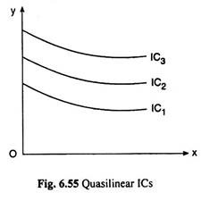
In order to understand quasilinear preferences, suppose that a consumer has indifference curves (ICs) that are vertical translates of one another as given in Fig. 6.55. This means that all of the ICs are just vertically shifted versions of one IC.
It follows that the equation of an IC here takes the form:
y = k – v (x) (6.119)
where U = U (x, y) (6.120)
is the ordinal utility function of the consumer.
Eqn. (6.119) says that the height of each IC (i.e., y) is some function of x, viz., – v(x), plus constant k. Higher values of k give higher ICs. The significance of the minus sign before the function of x would be clear in the discussion below.
The natural way to label the ICs here is with k—roughly speaking, the height of the IC along the vertical axis. Solving for k and setting it equal to ordinal utility, we have
U (x, y) = k = v (x) + y. (6.121)
In this case, the utility function is linear in the quantity of good Y, but (possibly) non-linear in the quantity of good X; hence the name quasilinear utility, meaning “partly linear” utility. Specific examples of quasilinear utility would be
U = √x + y (6.122)
and U (x, y) = In x + y (6.123)
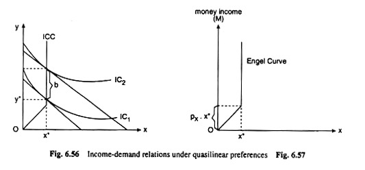
Quasilinear utility functions are not particularly realistic, but they are very easy to work with. Let’s first see what happens if the budget line is shifted outward. In this case, if an IC is tangent to the budget line at a bundle (x*, y*), then another IC must also be tangent at money income (M) (x*, y* + b) for any constant b.
Therefore, an increase in income does not change the demand for good X at all, and all the extra income goes entirely to the consumption of good Y.
If preferences are quasilinear, sometimes say that there is a zero income effect for good X. Thus, the consumer’s income-consumption curve and the Engel curve for good X are both vertical straight lines as shown in Figs. 6.56 and 6.57. As change in income, demand for good X remains constant. This is true of course, for his money income ≥ px.x*, where px is the price of good X.
Price Effect, Income Effect and Substitution Effect under Quasilinear Preferences (QLP):
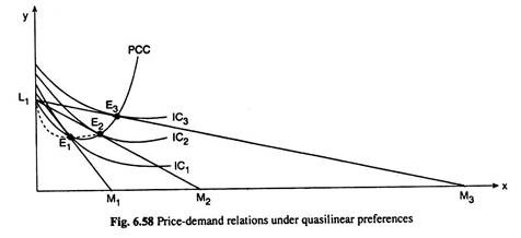
PCC under QLP for price-changes of good X has been shown in Fig. 6.58. Here the initial budget line of the consumer is L1M1 and the initial equilibrium point is E1.
As the price of X falls, ceteris paribus, the budget line rotates from L1M1 to L2M2 to L3M3… and the consumer’s equilibrium point moves from E1 to E2 to E3,…. Join the points L1 E1 E2, E3,.. ., by a curve, the consumer’s PCC under QLP for price changes of good X is obtained.
The price-effect, income effect and substitution effect under QLP have been explained in Fig. 6.59. In this figure, the consumer’s initial budget line is L1M1 and his initial equilibrium point is E1 on IC1. At this point he purchases OA1 of good X and OB1 of good Y. Suppose, the price of good X falls, ceteris paribus.
As a result, the consumer’s budget line would rotate anticlockwise about the point L1—it would now be, say, L1M2. In this new situation, the consumer would be in equilibrium at the point E2 where his budget line L1M2 would touch a higher IC, viz., IC2, and he would now purchase a larger quantity of X, viz., OA2 and a smaller quantity of Y, viz., OB2.
He is now on a higher IC since his real income has improved. Here the movement in his equilibrium point from E1 to E2 is the price effect movement—his purchase plan changes from the point E1 to the point E2 on account of the price-effect (PE). Specifically, here PE for good X has been + A1A2 and that for good Y has been – B1B2.
Now break up this price effect (PE) into a substitution effect (SE) and an income effect (IE). In order to isolate the SE portion of the PE, let’s apply the compensating variation in consumer’s money income, i.e., let’s notionally reduce his money income by M2G in terms of good X or L1F in terms of good Y, so that his budget line now would have a parallel shift to FG and it would touch IC1 at some point like E3; this indicates that the consumer’s real income now has been brought back to its initial level while there has been a change in the relative prices of the goods.
Therefore, by definition, the movement from point E1 to E3 is the SE movement and due to SE, the consumer purchases A1A2 more of X and B1B3 less of Y, since X now is relatively cheaper and Y is relatively dearer. So the SE here has been obtained to be +A1A2 for good X and -B1B3 for good Y.
The IE portion of the PE is obtained if the consumer is given back the amount of compensating variation in income. As this is done, the consumer’s budget line would have a parallel rightward shift from FG to L1M2.
Under QLP, his equilibrium point would now move vertically from point E3 to point E2. This movement is the IE movement. Since the movement is vertical, IE for good X is zero, as it should be under the QLP under consideration, and the IE for good Y has been +B2B3 in Fig. 6.59.
It may be now verified:
For good X, SE + IE = + A1A2 + 0 = + A1A2 = PE
and for good Y, SE + IE = – B1B3 + B2B3 = – B1B2 = PE
Therefore, it is verified, for both the goods:
PE = SE + IE.
