Let us make an in-depth study of the Consumption Function:- 1. Subject-Matter of the Consumption Function 2. Attributes of the Consumption Function.
Subject-Matter of the Consumption Function:
Consumption function is simply a name for the general income-consumption relationship embodied in the Psychological Law of Consumption given by Keynes.
Just as the demand curve shows the quantity of a commodity demanded at each possible price, so the consumption function shows the expenditure consumers will wish to make on consumer goods and services at each possible level of disposable income.
Thus, consumption function expresses the relationship between income (F) and consumption (C). In the income equation Y = C + I, the letter ‘C’ represents the amount of consumer expenditures made at a given level of income (Y). As the relationship between income (?) and consumption (C) is a functional one, we represent it as C =f(Y).
ADVERTISEMENTS:
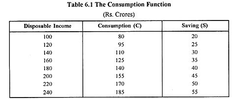
We know that at various levels of income there will be corresponding levels of consumption. We can prepare a schedule of the consumer expenditures at various levels of income-it is called the schedule of the propensity to consume or simply Consumption Function.
This is shown below in a tabular and diagrammatic form:
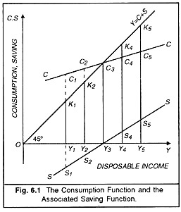
If we graph the tabular schedule of the propensity to consume, we get a curve which is the Consumption Function. Since as income rises, consumption expenditure rises, the curve representing the Consumption Function will rise from left upwards to the right. In Fig. 6.1 given below disposable income is shown on the horizontal and consumption spending (and saving is shown on the vertical axis. The 45° line shows the addition of consumption and saving to income.
ADVERTISEMENTS:
The line CC is sloping from left upwards to the right showing that as income rises consumption spending also rises but not as much as income. At a low level of disposable income such as OY2 consumption is even more than income resulting in dis-saving to the extent of C1K1 (= Y1S1)- As income rises to the level OY2, consumption rises to Y2K2 but still people spend more than their income resulting in negative saving of C2K2 (=Y2S2). At income level OY3, people wish to consume the whole of their income which means zero saving the CC line intersects the 45° line and the saving curve SS cuts the horizontal axis.
As income rises further to OY4 and OY5 levels, consumption spending is less than the income levels resulting in positive saving of Y4S4 and Y5S5 respectively. Thus the consumption function CC shows that as income increases, consumption increases and the saved amount also increases.
Consumption function is the central concept of Keynes’ General Theory. It brought to light the basic fact that in a free-enterprise economy, consumption spending depends, in the short run, on the level of income. Other factors also affect consumption but are stable in the short period with which Keynes was concerned. As income level rises consumption spending also rises but at a slower rate than income with the result that income unspent on consumption-saving-goes on accumulating. If a level of income is to be maintained, the saving out of it must be invested.
ADVERTISEMENTS:
This may always be possible. In this way, through the Consumption Function the problem of income theory is brought forth. With this knowledge of the consumption function, we study its two technical attributes-the Marginal Propensity to Consume and the Average Propensity to Consume.
Attributes of the Consumption Function:
1. Marginal Propensity to Consume (MPC):
Marginal propensity to consume denotes the ratio of a small change in consumption as a result of a small change in income. In other words, it refers to the marginal increase in consumption (∆C) as a result of marginal increase in income (∆Y) and is expressed as MPC ∆C/∆Y [the symbol (A) stands for small or marginal increase in income and consumption], Keynes believed in his psychological law of consumption that with an increase in income, consumption does increase but by less
than the increase in income. In other words, the ratio of the increase in consumption to the increase in income is always less than one i. e., ∆Y (increment in income) is always greater than OC (increment in consumption). Since ∆Y is greater than ∆C, ∆C/∆F will be less than unity. ∆C/∆Y is called Marginal Propensity to Consume.
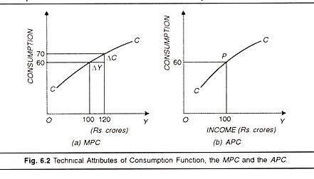
In technical language, it means that the marginal propensity to consume is less than one (less than unity). We can explain the concept with the help of a numerical example. Suppose Y increases from Rs. 100 crorcs to 120 crorcs ; the increment in income AY is Rs. 20 crores. Corresponding to this increase in income, consumption may increase from Rs. 60 crores to Rs. 70 crores, increment in consumption (∆C) being Rs. 10 crores. Hence MFC is ∆C/∆Y i.e., 10/20 = 1/2 = 0.5 (less than unity).
It is found out by dividing marginal change in consumption (∆C) by marginal change in income (∆F). The derivation of MPC of a consumption function at a particular level of income is shown graphically in Figure 6.2 (a) above. ∆C/∆Y is shown in the diagram as the coefficient of ∆C/∆Y which is 10/20=0.5. Geometrically, it is the slope of the consumption function at a particular point.
The concept of MPC is of utmost importance as it tells us how an increment in income will be divided between consumption and saving. In fact, the Psychological Law of consumption can be stated as that MPC is always less than one.
2. Marginal Propensity to Save (MPS):
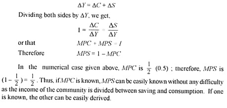
The complement of MPC is Marginal Propensity to Save, written as MPS, It can be easily derived from MPC. We know that an increment in income is divided between DC and an increment in saving ∆S.
3. Average Propensity to Consume (APC):
The other technical attribute of the consumption function is Average propensity to consume. Average propensity to consume is the ratio of absolute consumption to absolute income at a particular time and is expressed as C/Y.
APC shows the proportion of aggregate consumption to aggregate income. For example when income is Rs. 100 crores and consumption expenditure is Rs. 60 crores. APC is 60/100 (C/y) = 3/5=0/6 or 60%. Thus, the value of APC for any income level may be found by dividing consumption by income. Prof. Hansen has estimated APC in the United States in normal times to be at 88%. The APC is shown in figure 6.2 (b) on the previous page.
In this figure we measure income along the horizontal and consumption along the vertical axis. The ratio of consumption C to income Y (C/Y) shows the PC to be 0.6 or 60%. In terms of our diagram, APC implies a point on the C curve which indicates the ratio of Consumption to income. The C curve is made up of a series of such points. Every points has its own APC measured by the ratio of its perpendicular distances from the horizontal and vertical axis. APS also declines as it moves along the C curve to the right as seen from the flattening of the C curve measuring the declining proportion of community’s consumption to income.
The economic significance of APC is that it tells us what proportion of the total cost of a given output, as a result of planned employment, may be expected to be recovered from the sale of consumer goods alone so that the rest has to be made good by the sale of capital goods.


