Consumption: Importance, Keynesian Function and Optimisation

Let us make an in-depth study of Consumption. After reading this article you will learn about: 1. Importance of Consumption 2. The Keynesian Short-Run Consumption Function 3. Optimisation 4. Effect of Changes in Income on Consumption 5. Effect of Changes in the Real Interest Rate on Consumption.

Importance of Consumption:

The consumption function is of considerable importance for macroeconomic analysis and policy formulation primarily because households’ consumption decisions affect the way the economy as a whole behaves — both in the short run and in the long run.

Household consumption decision is crucial for short-run analysis because consumption expenditure of households largely determines aggregate demand which, in its turn, determines the level of employment and national income. The consumption decision is crucial for long-run analysis because Of its role in determining the rate of growth of the economy.

Since the publication of Keynes’s General Theory in 1936 many economists-such as Arthur Smithies, Simon Kuznets, James Duesenberry, Robert Ando, Franco Modigliani, R. E. Brumberg and Milton Friedman have written consistently about consumers’ behaviour patterns and suggested alternative ways of interpreting the data on consumption and income.

Studies show that the ratio of consumer expenditure to income varies inversely with the level of income but on average this ratio does not tend to fall as income rises over a long period.

The relation between income and consumption has drawn the attention of economists for a long time. However the relation was first studied in a systematic way by J. M. Keynes in 1936. And it was Keynes who developed a major microeconomic concept known as the consumption function.

The consumption function is a statement of the general relation between the dependent variable, consumption expenditure and the various independent variables determining consumption such as current disposable income and income from previous periods and wealth.

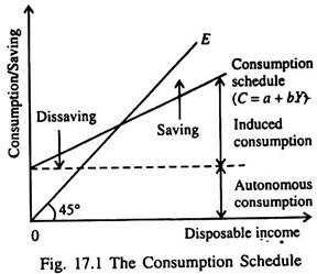
At low levels of disposable income households consume more than their current income, drawing on past saving, borrowing or selling assets in order to maintain consumption at some desired minimum income level (autonomous consumption). At higher levels of disposable income they consume a part of their current income and save the rest.

A simple consumption schedule takes the linear form C = a + bY, where C is consumption and a is the minimum level of consumption expenditure at zero disposable in­come (autonomous consumption). Thereafter consumption expenditure increases as income rises (induced consumption), and b is the pro­portion of each extra rupee of disposable income which is spent.

The 45° line 0E in Fig. 17.1 shows what consumption would have been had it exactly matched disposable income. The dif­ference between 0E and the consumption sched­ule indicates the extent of dissavings or savings at various income levels. The slope of the con­sumption schedule is equal to the marginal propensity to consume.

Keynes made the consumption function central to his theory of economic fluctuations (business cycles). In A. H. Hansen’s view, the consumption function lies in the heart of Keynesian economics.

The Keynesian Short-Run Consumption Function:

Keynes made predictions about consumption function on the basis of introspection and casual observation, not on the basis of actual studies of the behaviour of consuming units.

Three points may be noted in this context:

1. Value of MPC:

Keynes’ most important hypothesis is that the MPC — the amount consumed out of an additional rupee of income — lies between zero and one. His fundamental psychological law is that people, in general, and, on an average, are disposed to increase their consumption as their income increases, but by less than the amount by which income increases.

This means that a part of additional income is spent on consumption goods and a part is saved.

2. Fall in APC:

Keynes also postulated that the APC — the ratio of total consumption to total income — falls with every increase in income. To him saving is a luxury. This is why he expected the rich to save a higher proportion of their income than the poor.

3. Secondary Role of Interest Rate:

Income is the primary determinant of consumption. Interest rate plays a secondary role in determining individual consumption spending. On this point Keynes differed from the classical economists who thought that a higher interest rate encourages saving and discourages consumption.

On the basis of these three hypotheses the Keynesian consumption function can be expressed as:

C = a + bY, a > 0, 0 < b < 1

Three properties:

This consumption function has all the three properties that Keynes had highlighted:

1. Since MPC(b) lies between zero and one, higher income leads to both higher consumption and higher saving.

2. Here APC = C/Y = a/Y + b. As Y rises, a/Y falls. So APC falls. As Y rises and APC > MPC.

3. The interest rate is not included in the consumption equation. So it is not a determinant of consumption.

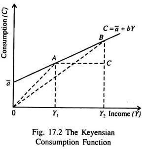
All these three properties of Keynes consump­tion function are shown in Fig. 17.2. In the short run, consumption has an autonomous (income- independent) component. This is why the con­sumption line C = a̅ + bY does not start from the origin. It has an intercept (a̅) on the vertical axis.

The MPC is the slope of the consumption function and in Fig. 17.2 it is BO AC = AC/AK Here APC or C/Y equals the slope of a line drawn from the origin to a point on the consumption function, i.e., AY₁/OY₁ when income is OY₁, and BY₂/OY₂ when income is OY₂.

In the short run MPC < APC due to presence of the autonomous component: MPC=b and APC = a/Y + b . Since a̅ > 0 and Y > 0, a̅/Y > 0. Therefore MPC < APC.

According to Keynes’s absolute income hypothesis an individual’s consumption depends on his own (absolute) income. This happens only in the short run.

Optimisation in Consumption:

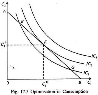
A rational consumer seeks to choose the best combination of C₁ and C₂ by being able to reach the highest attainable indifference curve permitted by the intertemporal budget line, which measures the total resource available to him over the two periods.

In Fig. 17.5 the budget line is tangent to IC₂ at point F. This is the optimum point showing the best combination of consump­tion in the two periods that is permitted by the inter temporal budget constraint (line).

At the optimum point F the slope of highest attainable indifference curve IC₂ (i.e., MRS) equals that of the budget line (i.e., 1 + r). The consumer chooses con­sumption in periods 1 and 2 such that the desired rate of substitution = the actual rate

or, MRS = 1 + r.

Effect of Changes in Income on Consumption:

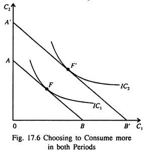
An increase in income in either period 1 or period 2 shifts the budget constraint to the right as shown in Fig. 17.6. This permits the consumer to attain a higher indifference curve and choose a better combination of C₁ and C₂ by moving from point E to F.

Thus he is able to consume more in both periods. As Y = Y₁ + Y₂ rises, so does C = C₁ + C₂. Here we assume that both C₁ and C₂ are normal goods, i.e., both increase when y increases.

Consumption Smoothing Over Time:

So the prediction here is that irrespective of whether the increase in income occurs in period 1 or 2, the consumer spreads it over in both periods. This type of behaviour is known as consumption smoothing. Even if future income is discounted at the market rate of interest the timing of income, i.e., when income is received does not affect today’s consumption level.

The reason is that the consumer can borrow and lend between periods. This simply means that consumption depends on the present value of current and future incomes — that is, on

PV (Y₁ + Y₂) = Y₁ + Y₂/1 + r

This conclusion is completely different from the one reached by Keynes who made a timeless analysis of consumption behaviour. According to Keynes, a person’s current consumption depends only on his current income. In contrast, in Fisher’s model, an individual’s consumption depends on the resources he expects over his lifetime (i.e., his total income or endowment).

Effect of Changes in the Real Interest Rate on Consumption:

A change in the real interest rate alters the consumer’s choice, depending on whether he is initially saving or borrowing. Here we assume that the consumer is a saver and not a borrower. However, the same analysis can be slightly modified to analyse the case where the consumer is borrowing.

Case 1: The Consumer is a Saver:

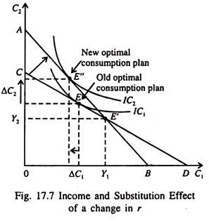
Fig. 17.7 shows that an increase in r rotates the consumer’s intertemporal budget line around the point e’ (corresponding to Y₁, Y₂) and thereby alters the value of consumption he chooses in both periods. As the interest rate increases, the budget line becomes steeper. And as the consumer moves from point E to E”, C₁ falls and C₂ rises. And he gets a higher level of utility by doing that.

The movement from E to E” can be decom­posed into two parts — the income effect and the substitution effect.

Income effect:

The income effect measures the change in consumption which occurs when the consumer moves to a higher indifference curve. In this case the consumer is a saver because C₁ < Y₁. So an increase in r makes him better off and moves him to a higher indifference curve. If both C₁ and C₂ are normal goods, he will increase both C₁ and C₂ and spread the gain in total welfare over both periods.

Substitution effect:

The substitution effect measures the change in consumption which results from the change in the relative price of C₁ and C₂. A rise in r makes C₂ less expensive than C₂. The reason is easy to find out. Since r on saving is higher, the consumer is required to sacrifice less C₁ to obtain every extra unit of C₂. So the substitution effect of a rise in r is to induce the consumer to consume more in period 2 and less in period 1.

The end result:

The consumer’s choice depends on both the effects. The two effects originating from a rise in r together increase C₂. But as far as C₁ is concerned, the two effects go in opposite directions. Thus whether a rise in r increases or lowers C₁ is not clear.

Case 2: The Consumer is a Borrower:

In Fisher’s model the ability to borrow enables a consumer to consume more than what his current income permits. Borrowing money to consume means that the consumer is using a portion of his future income today. But all people cannot borrow. So it is interesting to see how Fisher’s analysis changes in the presence of borrowing constraint.

Constraints on Borrowing:

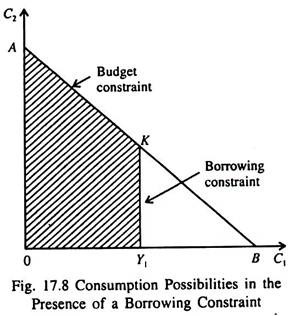
If the consumer cannot borrow his current consumption has to be less than or, at least, equal to his current income. So we get

C₁ < Y₁

This inequality is known as a borrowing constraint or a liquidity constraint.

Now the consumer’s choice is restricted by two constraints, viz., the budget constraint and the borrowing constraint. Fig. 17.8 shows the consumer’s choice in such a situation. The shaded area OAKY₁ — which satisfies both the constraints shows the combination of C₁ and C₂ the consumer can choose.

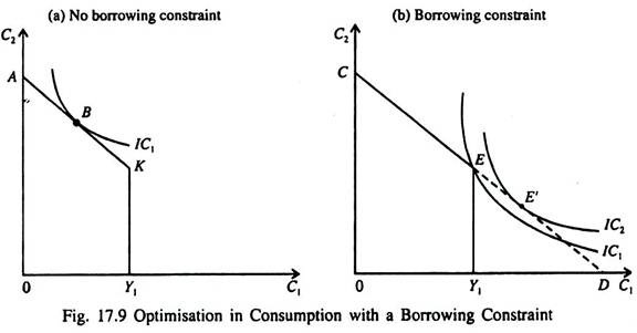
Fig. 17.9 shows the consumer’s decision in the presence of this borrowing constraint. As shown in part (a) if the consumer wants to consume less than what he earns in period 1 then the borrowing constraint does not affect his consumption decision in either period.

But, as part (b) shows if the consumer wants to consume more in period 1 than he earns, he can consume as much as is permitted by Y₁ and he cannot consume more due to the borrowing constraint. So even if he prefers to move to point E’ which is on a higher indifference curve the borrowing constraint forces him to stay at point E, which is his best available chose. In other words, in the presence of the borrowing constraint, C₁ = Y₁.

Thus when borrowing constraint is present, there are two consumption functions. In case of those consumers who do not face any borrowing constraint, consumption in both periods depends on the present value of lifetime income, Y₁ + [Y₂/( 1 + r)].

For others, who face such constraint, the consumption function is C₁ = Y₁ and C₂ = Y₂. Thus only for those consumers who are not able to borrow, consumption depends only on current income. Thus in the presence of borrowing constraint the Keynesian analysis is more relevant than the Fisher two- period analysis.