Shapes of Various Short Run Cost Curves (With Diagram)

Let us make an in-depth study of the shapes of various short run cost curves.

Short Run Cost Curve # Average Fixed Cost (AFC):

Average fixed cost is the fixed cost per unit of output.

This is obtained by dividing the total fixed cost by the level of output:

AFC = TFC/Q, where Q = output

As output increases and TFC remains fixed, AFC declines continuously. As the same volume of fixed cost is divided by the – larger volume of output, AFC must decline. Further, the AFC curve is a rectangular hyperbola in the sense that all rectangles formed by AFC are of equal sizes. The AFC curve is asymptotic to both the axes. This means that it touches neither the horizontal axis nor the vertical axis.

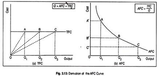
Fig. 3.13 illustrates the derivation of AFC curve from the TFC curve. In Fig. 3.13(a), we have drawn TFC curve parallel to the output axis. Here the output OQ₁, OQ₂ and OQ₃ have been measured in such a way that OQ₁ = Q₁Q₂ = Q₂Q₃.

Since AFC = TFC/Q, AFC is given by the slope of a ray from the origin to a point on the TFC curve. We have chosen points A, B and C on the TFC curve and on all these points we have drawn rays OA, OB and OC.

Consider output OQ₁. Corresponding to this output level, AFC is the slope of the ray OA, i.e., AFC = Q₁A/OQ₁. Similarly, for output OQ₂, AFC = Q₂B/OQ₂and for output OQ₂, AFC = Q₃C/OQ₃. As fixed costs do not change, one can say that Q₁A = Q₂B = Q₃C.

TFC curve in panel (a) has been drawn in such a way that OQ₂ = 2OQ₁ and OQ₃= 3OQ₁.Thus, AFC for OQ₂ output becomesQ₂B/OQ₂ = Q₁A/2OQ₁ = ½ (Q₁A/OQ₁)= ½ AFC for output OQ₁. This is shown in panel (b) by the difference in OA and OB—more specifically OB’ = ½OA’.

Likewise, AFC for OQ₃ output is Q₃C/OQ₃ = Q₁A/3OQ₁ = ⅓ (Q₁A/OQ₁) = 1/3 AFC for output OQ₁. This means OC’ = 1/2 OA’. In this way, AFC is obtained.

Here all the rectangles are of equal size since fixed costs do not change. For instance, for OQ₁ output, AFC multiplied by output OQ₁ gives us TFC. Thus, OA’AQ₁ rectangle is the TFC for output OQ₁. For output OQ₂ and OQ₃, though AFC declines, fixed cost remains constant because rectangle 0B’BQ₂ =rectangle OC’CQ₃.

In short, AFC is a rectangular hyperbola.

Short Run Cost Curve # Average Variable Cost (AVC):

AVC is the variable cost per unit of output. AVC is obtained by dividing TVC by the level of output:

AVC = TVC/Q

If AVC is plotted on a graph paper, one will find that, initially, AVC will decline, will reach a minimum, and, thereafter, it will rise. Thus, the AVC curve is U-shaped. The reason is the law of variable proportions. In other words, there is a relationship between costs of production and input productivity.

Let us assume that labour is the only variable input and, therefore, the only variable cost is labour cost—which is nothing but quantity of labour multiplied by wage rate, i.e.,

TVC = L.W

We know that

AVC = TVC/Q = W.(L/Q)

But output divided by labour, i.e., Q/L is the average product (AP), i.e., AP = (Q/L)

Hence, AVC = W. (1/Q/L)

Or, AVC = W. (1/AP_L)

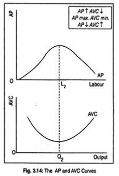
Thus, AVC is the wage rate multiplied by the reciprocal of AP. Since, at the initial stage, AP rises, then reaches maximum and then declines, AVC must, therefore, fall, reach a minimum, and rise thereafter. In other words, the movement of the AP curve is just the reverse of the AVC curve or AVC is the mirror image of the AP.

Fig. 3.14 shows the inverse relationship between AP and AVC curves. The upper panel shows that, as use of labour increases, AP rises and, hence, AVC declines. At OL₂ level of employment, since AP is maximum, AVC at the OQ₂ output must be minimum. Beyond OL₂ amount of labour, as AP declines, AVC rises. Hence, the AVC curve is U-shaped.

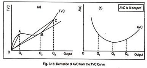
How the AVC curve is derived from the TVC curve has been explained in Fig. 3.15. AVC at each level of output is given by the slope of a line drawn from the origin to the corresponding point on the TVC curve. For example, AVC at output OQ₁ is the slope of the ray OA from the origin. AVC at output OQ₂ is the slope of the line OB.

The slope of the ray steadily diminishes until OQ₂ is produced. To the right of OQ₂, the slope rises. In other words, the slope of TVC at output OQ₃ is larger than TVC at output OQ₂. That is why the slope of the AVC curve (drawn in panel b) is negative until output OQ₂ is attained. At its minimum point, the slope is zero. After that point the slope becomes positive and the AVC curve rises, as shown in panel (b) of Fig. 3.15.

Short Run Cost Curve # Average Cost (AC or ATC):

AC is the total cost per unit of output. AC is obtained by dividing TC by output, i.e.,

AC = TC/Q = TFC + TVC/Q

= TFC/Q + TVC/Q = AFC + AVC

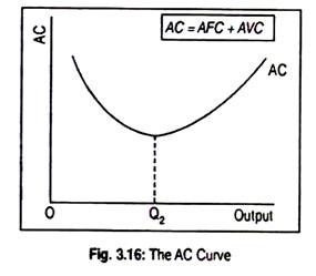
Thus, AC is the sum of AFC and AVC. Obviously, the shape of the AC curve (Fig. 3.16) is governed by the shapes of AFC and AVC curves. Truly speaking, the AVC curve is U-shaped. We know that, as output increases, both AFC and AVC decline, so AC must decline.

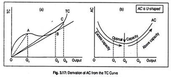
Though AVC now rises, the significant decline in AFC causes AC to decline more. And that is why AC’s minimum point comes later than the AVC’s minimum point. Anyway, up to OQ₂ level of output, AC declines. The level of output that corresponds to the lowest point of the AC curve is called the ‘optimal capacity’ or the ‘efficient scale’ of the firm.

If a firm produces less than the minimum point of the AC curve then it experiences ‘excess capacity’, and, if a firm produces beyond the minimum point of the AC curve, it experiences the ‘above capacity’. Beyond OQ₂ output, AC starts rising. This means that increase in output beyond OQ₂will lead to an increase in AVC.

In other words, the increase in AVC more than offsets the fall in AFC. That is to say, in this region of output, AVC becomes more strong than the AFC and AC continues to rise. Thus the AC curve is U-shaped. It is U- shaped due to the operation of the law of variable proportions.

Graphically, the AC curve is derived in the same way as AVC is derived from the TVC curve.

AC at each level is the slope of a line drawn from the origin to the corresponding point on the TC curve (Fig. 3 .17). The slope of the ray diminishes as one moves along the TC curve until B is reached. This means AC must decline till OQ₂ is attained. Thereafter, the slope of the line OC rises and the AC takes a positive slope. So, the AC curve is U-shaped.

Short Run Cost Curve # Marginal Cost (MC):

MC is the change in total cost attributable to a change in output. Thus, MC is an addition to the total cost. In symbols,

MC = ∆TC/∆Q

This means that MC is the difference between total cost for Qth and Q -1th unit of output. It is to be remembered here that, in the short run, fixed costs do not change. Here output changes due to change in the use of variable inputs. Thus by change in total cost we mean change in total variable costs only. Fixed costs do not have any bearing on MC. MC is independent of fixed cost. Thus,

MC = ∆TVC/∆Q

MC refers to change in total variable cost which results from a change in output.

We can prove this in the following way also:

MC = TC (Q) – TC (Q – 1)

= (FC + VC_Q)-(FC + VC_{Q – 1})

= FC + VC_Q -FC – VC_{Q – 1}

MC = VC_Q – VC_{Q – 1}

.^.. MC = ∆TVC/∆Q

MC is also defined as the reciprocal of MP multiplied by the price of the variable input. Suppose, labour is the variable input whose cost (i.e., wage cost) is the variable cost. Thus,

∆TVC = w. ∆L

Dividing this by ∆ Q, we obtain

MC = ∆TVC/∆Q = w. ∆L/∆Q

But, ∆Q/∆L = MP

.^.. MC = w. (1/MP) = w/MP

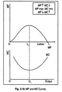
That is why it is said that the shape of the MC curve is governed by the shape of the MP curve. Since MP initially rises, reaches a maximum, and then declines, MC initially falls, reaches a minimum, and, thereafter, rises. So the MC curve is U-shaped due the operation of the law of variable proportions.

This has been shown in Fig. 3.18:

In this figure, as labour employment increases, MP initially rises and, consequently, MC falls as output rises. MP reaches maximum when OL₁ units of labour are used. Corresponding output level is OQ₁. Here MC becomes minimum.

Thereafter, employment of labour causes MP to fall even to zero or to become negative while MC continuously rises. Thus the MC curve is the reciprocal of the MP curve.

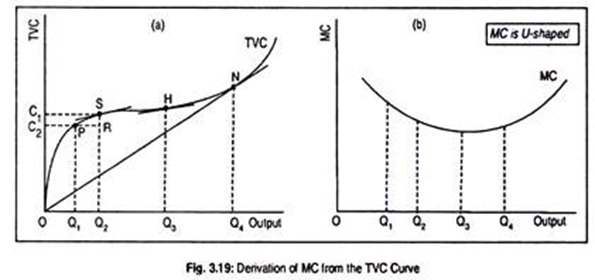
How MC is derived from the TVC curve can be known from Fig. 3.19. Graphically, MC curve is the slope of the TVC curve. The slope of a curve at any one of its points is the slope of the tangent at that point.

Suppose output increases from OQ₁ to OQ₂ and total cost increases from OC, to OC₂. We have drawn a tangent on the TVC curve at point S. Thus, MC at this point will be equal to the slope of the tangent, i.e.,

MC= OC₂ – OC₁/OQ₂ – OQ₁ = SR/PR

As one moves from P to S the distance between these two points becomes smaller and smaller and the slope of the tangent gradually declines till point S is reached. At this point, the slope of the tangent corresponding to the output OQ₃ is smallest and MC is the lowest.

This means that MC falls until OQ₃ is produced. The tangent at point N is also ray from the origin. However, as the slope of the tangent to the TVC curve rise after OQ₃ output, MC starts rising. Accordingly, the MC curve is U-shaped.

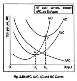
Now, all these short run cost curves can be represented in a single diagram (Fig. 3.20). The AFC curve has been drawn as a rectangular hyperbola. The AFC curve is declining steadily. The AVC curve is U- shaped. MC passes through its minimum point (N).

AC being the sum of AFC and AVC, AC curve lies above both the AFC and AVC curves. Again, MC passes through the minimum point of the AC (point P). Notice, AVC and AC get closer as output rises since AFC continuously declines as output rises. Like the AVC and AC, the MC curve is also U-shaped.

MC equals both AVC and AC at their minimum points. Further, MC lies below both AVC and AC over the range in which these curves fall; and it lies above them when they are rising It is to be kept in mind that all the cost curves—except the AFC curve— are U-shaped.