Break-Even Analysis : Methods, Margin of Safety and Uses

Break-even analysis is a method that is used by most of organizations to determine, a relationship between costs, revenue, and their profits at different levels of output’.

It helps in determining the point of production at which revenue equals the costs. Break-even analysis is also called as profit contribution analysis.

Some of the popular definitions of break-even analysis are as follows:

According to Matz, Curry and Frank, “a break-even analysis indicates at what level, cost and revenue are in equilibrium.”

According to Keller and Ferrara, “the break-even point of a unit of a company is the level of sales income which will equal the sum of its fixed costs and its variable costs.”

According to Charles T. Homogreen, “the break-even point of activity (sales volume) is where total revenue and total expenses are equal. It is the point of zero profit and zero loss.”

The important aspect of understanding break-even analysis is the break-even point at which there is no net loss or gain of an organization as expenses equals revenue.

The break-even analysis is done under two conditions, which are as follows:

i. Linear cost and revenue relationship

ii. Non-linear cost and revenue relationship

On the basis of these two conditions, there are a number of methods for performing break-even analysis.

Some of these methods are shown in Figure-16:

The methods of break-even analysis (as shown in Figure-16) are explained as follows:

i. Graphical Method:

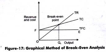
Shows a linear break-even analysis. When price of a product remains the same, the organization expands its production, thus, total revenue is linear to the output.

Let us learn this method through Figure-17:

As shown in Figure-17, TFC is equals to FE, which is a fixed cost line. The vertical distance between TC and TFC line equals TVC. As quantity of output increases, the vertical distance between TC and TFC increases. This implies that TVC increases with change in TC and TFC.

Until Qb of the quantity is produced, total cost exceeds the total revenue, which implies that an organization will suffer losses if it produces less than Qb. At Qb output level, total revenue equals total cost. At this point, an organization never makes profit nor loss implying that it is a break-even point. Thus, Qb is a break-even level of output. Producing more than Qb will be profitable for organizations as TR is greater than TC.

ii. Algebraic Method:

Helps in decision making problems of the organization. We know that profit is equal to difference between total revenue and total cost.

π = TR – TC

TR = P*Q

TC = TVC + TFC

TC = AVC*Q + TFC (TVC is the variable cost per unit multiplied by the output produced and sold)

Let Qb is the break-even quantity at which TR = TC.

TR = TC

P. Qb = TFC + AVC. Qb

P.Qb – AVC.Qb = TFC

(P – AVC)Qb = TFC

Qb = TFC/ (P-AVC)

Thus, from the above equation, it can be said that the break-even quantity of output is determined by TFC, price and variable cost per unit of output.

iii. Contribution Analysis:

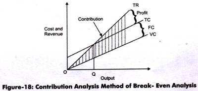
Refers to the analysis of incremental or additional revenue and costs of a business. Contribution is the difference between total revenue and variable costs.

Let us discuss this through Figure-18:

Fixed costs are addition to variable costs. Thus, TC line is parallel to the variable costs line. In the Figure-18, OQ is the break-even point. TC minus VC equals FC. Below OQ, contribution is less than fixed cost whereas beyond OQ, contribution exceeds faxed cost. The shaded portion between TR and VC is the contribution.

Profit volume (PV) ratio:

Refers to another method to find break-even point. The formula for profit volume ratio is:

PV ratio = (S-V)/S* 100

S = Selling price

V = Variable costs

Margin of Safety:

The margin of safety is defined as a difference between sales at a break-even point and total actual sales. This term was given by Benjamin Graham and David Dodd in their book, Security Analysis. The margin of safety is useful when the sales of organizations are at risk.

There are three measures of margin of safety used given as follows:

Margin of safety = (profit * sales)/PV ratio

Margin of safety = profit/PV ratio

Margin of safety = (S_a – S_b) *S_a * 100

Sa = Actual sales

Sb = Sales at break-even point

Let us study the working of margin of safety as follows:

TR = 20 Q

TC= 100 + 10 Q

Sa = 40

We know that TR = TC at break- even point.

Let’s substitute Sb in place of Q in TR and TC functions.

TR = 20 Sb

TC = 100 + 10 Sb

TR = TC (at break-even point)

20Sb = 100+ 10 Sb

Sb = 10

Thus, margin of safety = (20 – 10)/20 * 100 = 50%

The margin of safety can be increased by the following methods:

i. Increasing tire selling price, provided sales are not affected (this is possible in case of inelastic demand of product)

ii. Increasing production and sales up to the capacity of the plant

iii. Reducing the fixed expenses or variable expenses

Uses and Limitations of Break-Even Analysis:

In break-even analysis; the costs of an organization are compared with the level of sales volume to find out the point at which the business likes non-profit no loss situation. It is a useful tool for management to make various business decisions and deal with uncertainty.

The uses of break-even analysis are as follows:

i. Helps in determining the sales volume

ii. Forecasts profits if estimates of revenue and cost are available

iii. Helps in appraising the effects of change on volume of sales and cost of production

iv. Assists in making choice of products and determining product mix

v. Highlights the impact of increase or decrease in the fixed and variable costs

vi. Studies the effect of high-fixed costs and low variable costs

vii. Makes intra-firms profitability comparisons

viii. Helps planning of cash requirements for organizations effectively

In spite of its uses, the limitations of break-even analysis are as follows:

i. Fails to be applied effectively in the multiple products situation

ii. Fails to be implemented in the situation where cost and price cannot be ascertained and where historical data is not available

iii. Assumes fixed costs to be constant

iv. Assumes that quantity of goods produced is equal to the quantity of goods sold, which may not be always true

v. Ignores changes in selling prices

vi. Ignores market conditions.