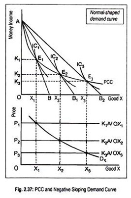
Let us learn about the construction of demand curve from the price consumption curve.
Assume that a consumer purchases good X from his limited money income. In the upper part of Fig. 2.37, we have drawn price consumption curve (PCC). In the upper panel, the horizontal axis measures quantities of X while the vertical axis measures money income instead of the usual practice of measuring another good, say Y.
Here money income may be treated as a composite good whose price is assumed to be constant. Further, the indifference curve drawn here shows combinations of the two goods X and money income (or a composite good) that give the same level of satisfaction.
ADVERTISEMENTS:
Suppose, a consumer has a money income of OA. With this given income he purchases different quantities of X at different prices. With income OA, the consumer can purchase maximum OB amount of X. Thus, AB is the initial budget line. As the line AB is tangential to IC1 at point E1 the consumer reaches equilibrium there.
If the price of X falls, the budget line would shift to AB1 and the new equilibrium would be achieved at point E2. E3 is another equilibrium point when the budget line is AB2 following a decline in the price of X. By connecting all these equilibrium points E1, E2 and E3, we get price consumption curve (PCC).
This curve shows various quantities of X that a consumer is willing to purchase at various prices but does so indirectly through total expenditure incurred on this commodity. To derive the price of X that is charged in the market, we have to divide the total expenditure of X by the respective quantities of X that the consumer would purchase.
Suppose, the initial equilibrium point is E1 and the equilibrium quantity that is purchased is OX1. This means that the consumer, out of his total money income OA, spends AK1 to purchase OX1 of X. Thus, the price of X per unit becomes K1A/OX1. This price is shown as OP1 in the bottom part of the Fig. 2.37.
ADVERTISEMENTS:
Similarly, at equilibrium point E2, the consumer spends AK2 to buy OX2 of X. Thus, the price per unit of X is OP2 (= K2A/OX2), shown in the lower part of the figure. Likewise, we find out the price at point E3. As the consumer spends AK3 to buy OX3 amount of X, the price per unit comes to AK3/OX3 or OP3. This has been shown in the lower part.
Thus, the consumer purchases OX1 at a price OP1, OX2 at a price OP2, and OX3 at a price OP3. By joining these equilibrium quantities we obtain the price-demand curve, DX, as a negative sloping curve. This means that, as the price of X falls, demand for X rises. Thus, good X is a normal or superior good. Anyway, for Giffen good, demand curve would be positive sloping.
