Aggregate Demand and Aggregate Supply with Flexible Price Level

Aggregate Demand and Aggregate Supply with Flexible Price Level!

Before analyzing the causes of inflation we need to explain aggregate demand-aggregate supply model with flexible price level.

Keynes in his income-expenditure analysis of income and employment assumed that price level remained constant. Concerned as he was with the unemployment problem of the economy under the grip of depression characterized by demand deficiency and excess capacity in the economy he validly assumed the price level to remain constant.

But during the Second World War and after, the problem of inflation, that is, continuous rise in general price level, was faced by many capitalist advanced countries. During this period Keynes himself explained inflation in terms of his inflationary gap which arises due to excess demand when the economy is working at its full capacity with full employment of workers.

Behind his analysis of inflation were aggregate demand and aggregate supply with flexible price level though he did not explicitly use the concepts of aggregate demand and aggregate supply curves with flexible price level. After Keynes it is with the concepts of aggregate demand and aggregate supply curves with flexible price level that inflation has been explained. It is therefore useful to explain these concepts before analyzing the problem of inflation.

Aggregate Demand (AD):

Let us first explain aggregate demand. Aggregate demand is the total desired quantity of goods and services that are bought by consumer households, private investors, government and foreigners at each possible price level, other things being held constant. Thus aggregate demand is not any quantity demanded at a particular price level but is a schedule of total output demanded at various price levels and is represented by a curve.

Thus aggregate demand has four components: consumption demand, private investment demand, Government purchases of goods and services and net exports. Thus, aggregate demand curve depicts the total output of goods and services which households, firms, and Government are willing to buy at each possible price level.

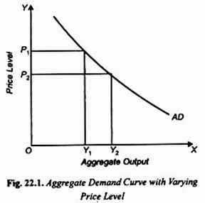
Thus aggregate demand curve shows the relationship between the total quantity demanded of goods and services and general price level. It is worth noting that aggregate demand curve (AD) differs from the ordinary demand curve of an individual commodity with which we are concerned in microeconomics though both slope downward to the right.

In case of a demand curve of an individual commodity when price of a commodity rises, it will tend to be substituted by other commodities which are its close substitutes resulting in fall in the quantity demanded of the commodity at a higher price. Thus, the slope of demand curve of an individual commodity depends mainly on the possibility of substitution between the commodities.

On the other hand, as we shall see below, the slope of aggregate demand curve depends on factors totally different from those that cause demand curve of an individual commodity to slope downward. We have drawn an AD curve in Figure 22.1 where on the horizontal axis we measure level of aggregate output and on the vertical axis we measure the general price level. As will be seen from Figure 22.1, aggregate demand curve AD slopes downward to the right.

It is important to note that the AD-AS model is unlike that of market demand- supply model of microeconomic theory. When we consider demand and supply in a particular market, say for cotton cloth, rise in its price will cause increase in its quantity supplied but in doing so resources will be withdrawn from other goods.

Such reallocation of resources between products and consequently rise in output of one product and fall in that of the other is not considered in macroeconomics where we are concerned with determination of aggregate output and total employment of resources in the economy as a whole.

Similarly, in macroeconomic model of aggregate demand and aggregate supply we study the determination of general price level which does not explain the relative prices of various products. We explain below in detail the concepts of aggregate demand (AD) and aggregate supply (AS) curves and their likely shape and factors determining them. We will also discuss some important controversial issues of macroeconomics with this AD-AS model.

Why does Aggregate Demand Curve Slope Downward?

Like the demand curve for an individual commodity, aggregate demand curve slopes downward but for different reasons. There are three factors responsible for downward-sloping aggregate demand curve.

First, as the general price level falls, the real value or purchasing power of money balances and monetary assets with the public increases. This makes the people feel better off or richer which induces them to increase their consumption which is an important component of aggregate demand. This is called real balance effect.

Second, with the fall in general price level, transactions demand for money falls which causes interest rate to fall. At a lower interest rate investment demand increases which also operates to bring about rise in aggregate demand at a lower general price level. This is called interest rate effect.

Thirdly, the fall in general price level makes exports of a country relatively cheaper leading to an increase in export demand for domestic goods produced in the economy. Besides, due to cheaper domestic goods as a result of fall in general price level, the people buy domestic goods instead of imported ones which reduces imports of a country. This causes net exports of the country to rise and leads to the increase in aggregate demand at a lower price level. This is known as foreign trade effect.

Shifts in Aggregate Demand Curve:

Now, which factors cause aggregate demand curve to shift? We have drawn above aggregate demand curve AD in Fig. 22.1 keeping non-price factors such as government expenditure, taxes, autonomous investment, money supply as remaining fixed or constant. When there is change in any of these non-price factors, aggregate demand curve AD will shift.

For example, if there is increase in government expenditure without being matched by increase in taxes, aggregate demand curve will shift to the right indicating that at each price there will be more aggregate demand. Likewise, if RBI increases money supply in the economy, this will raise demand of the people for goods and services and cause a shift in aggregate demand curve to the right.

Aggregate Supply:

Aggregate supply is the total output of goods and services that firms want to produce at each possible price level. Thus, like aggregate demand, aggregate supply is the whole schedule of total quantities of aggregate output that firms in the economy are willing to produce at each possible price level and can be represented by an aggregate supply curve.

It is worth noting that aggregate supply is the outcome of the decisions of all producers in the economy to hire workers and buy other inputs for production of goods and services for selling them to consumers, other producers, government as well as for exporting them to other countries.

It may be noted while drawing aggregate supply curve that depicts relationship been quantities of aggregate output that are produced for sale in the market by the firms in the economy at various price levels, all other factors that affect aggregate supply being held constant.

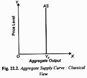
There is a lot of disagreement among economists about the shape of aggregate supply curve. The classical economists assumed that there normally prevailed full-employment of resources in the economy. According to them, if at any time there is deviation from this full-employment level, the wages, interest and prices quickly and automatically adjust and change to restore equilibrium at the full-employment level.

Thus, in the classical theory, the aggregate supply curve of output is perfectly inelastic (i.e. a vertical straight line) at the output level corresponding to full-employment level of resources. This aggregate supply curve relating aggregate supply with price level of the classical theory of income and employment is shown in Figure 22.2 by a vertical AS curve.

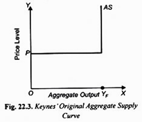
On the other hand, Keynes considered the situation of economic depression when the economy was operating before the level of full employment of resources. He further believed that in such a situation money wage rates were sticky i.e. remained constant. He further assumed that average and margined products of labour remain constant when more of it is employed following the increase in aggregate demand.

With these assumptions, more aggregate output is produced and supplied at the given price level in response to increase in aggregate demand. But when full employment of labour and capital stock is attained and aggregate demand further increases, aggregate supply curve being unable to increase any more, it is the price level that will rise in response to the increase in aggregate demand Keynes’ aggregate supply curve depicting the relationship between price level and the aggregate production (supply) during the period of depression and involuntary unemployment when there is a lot of excess capacity in the economy is shown in Figure 22.3 where it will be seen that aggregate supply is a horizontal straight line (i.e. perfectly elastic) up to full-employment output Y_f showing thereby that more is produced and supplied at the same price level OP but corresponding to full-employment level point Y_f it becomes vertical.

It may however be noted that Keynes recognized that as the aggregate supply approaches close to the full-employment level, the cost of output per unit tends to rise due to the rise in wage rate and also due to diminishing returns to extra factors employed. But, according to Keynes, the rise in price at full-employment level before full employment or less than capacity output will not be much.

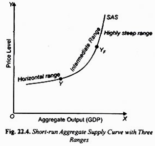
It is evident from above that shape of aggregate supply curve has been a highly controversial issue. However, there is now a general consensus among modern economists that when the economy is working substantially below capacity, that is, at times of depression or severe recession, more can be produced without much rise in marginal cost of production and therefore the aggregate supply curve is nearly flat.

This first range is therefore called horizontal range. With the given stock of capital (i.e. plant and equipment) when output is expanded beyond this range the diminishing returns and rising marginal costs occur which ultimately cause the aggregate supply curve to slope
upward gently.

Thus there is a part of gently rising short-run aggregate supply curve which represents intermediate range of short-run aggregate supply curve. But as the firms in the economy approach near their capacity output, their marginal costs sharply rise which causes sharply rising aggregate supply curve. Beyond the level of capacity output, that is, when the given resources of the economy are fully employed, aggregate supply curve (AS becomes a highly steep curve).

Thus the short-run aggregate supply curve has segments or ranges:

(1) The horizontal range,

(2) The intermediate upward-sloping range, and

(3) The highly steep range.

This aggregate supply curve having three distinct segments is shown in Figure 22.4.

Shifts in Short-Run Aggregate Supply Curve:

In explaining the upward-sloping nature of short-run aggregate supply we stated that aggregate supply curve depicts the relationship between price level and aggregate output (i.e., real GDP), other factors such as wages, input prices, technology and indirect taxes that determine aggregate supply being held constant. Now, it is the changes in these other determining factors that cause a shift in the aggregate supply curve. We explain below the factors that cause a shift in aggregate supply curve.

Changes in Wage Rate:

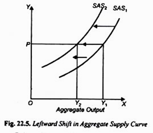
Change in wage rate of workers is an important factor that causes a shift in short-run aggregate supply curve. For example, when wage rate of workers increases, it causes a leftward shift in short-run aggregate supply curve. This is because increase in wages raises cost per unit of output. With a given price of output, higher wage rate means profit per unit of output will decline. As production becomes less profitable, it is likely that the firms will cut back on production and supply less output. Now when wage rate of workers increases, it causes a leftward shift in short-run aggregate supply curve as shown in Fig. 22.5.

Prices of Inputs:

Changes in prices of other inputs such as energy (for example, crude oil) and raw materials also bring about a shift in short-run aggregate supply curve. It is well known that increase in price of crude oil by OPEC in 1973 and again in 1979 affected aggregate supply by raising cost per unit of production. This caused a leftward shift in short-run aggregate supply curve as shown in Fig. 22.5 This leftward shift in the aggregate supply curve implies that at any given price level less output is supplied than before.

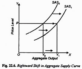
On the other hand, when price of crude oil falls as has happened at several occasions in the past, aggregate supply curve shifts to the right as is shown in Fig. 22.6 indicating that at any given price level more output will be produced and supplied than before.

Change in Technology. The change in technology is another important factor that causes a shift in aggregate supply curve. When there is improvement in technology, productivity of factors rises causing a fall in the unit cost of production. This brings about a rightward shift in aggregate supply curve showing that at any given price level more will be produced and supplied than before.

Business Taxes and Subsidies:

Increase in rates of business taxes such as excise duty, sales tax, customs duties raise per unit cost of production just as rise in wage rate. (Note that tax is considered as cost of production as it raises the supply price of output.) Thus, by levying business taxes or increasing their rates causes a leftward shift in the aggregate supply curve.

On the other hand, lowering of taxes as happened during the recent global slowdown (2007-09), caused by bursting of sub-prime housing loans bubble in United States, will cause a shift in the aggregate supply curve to the right. Provision of subsidies on products of various industries also causes a shift in the aggregate supply curve to the right.

Available Supply of Resources:

Lastly, a very important factor determining the position of aggregate supply curve is the available quantity of resources. When the available supplies of resources such as labour and capital increase, the short-run aggregate supply curve will shift to the right. As labour force grows and supply of capital is increased through investment, the short-run aggregate supply curve will shift to the right implying that more output will be produced for sale at any given price level.

Long-Run Aggregate Supply Curve:

In our above analysis we have explained the short-run aggregate supply curve with a variable price level. In the modern macroeconomic analysis the distinction is drawn between the long-run and short-run aggregate supply curve. Since classical economists who were concerned with determination of national income and employment in the long run, they considered the long-run aggregate supply.

The long-run aggregate supply is determined by three real factors such as availability of labour, the quantity of capital stock and the state of technology. In the long run price level is variable and the aggregate supply curve is vertical. On the other hand, Keynes considered the short-run aggregate supply which is perfectly elastic at the fixed price level in the period of depression.

However, in the modem or new Keynesian macroeconomics short-run aggregate supply curve slopes upward. Further, this short-run aggregate supply fluctuates over the course of a business cycle, that is, in different phases of the business cycle. The level of employment fluctuates around full-employment level and GDP fluctuates around the potential GDP.

Note that the quantity of real GDP when there is full employment of labour or, in other words, when unemployment is at its natural rate is known as potential GDP. Potential GDP depends on the given labour force and capital stock when they are fully employed or used, given the state of technology. We explain below in detail the concept of long-run aggregate supply and short-run aggregate supply.

Long-run Aggregate Supply:

The long-run aggregate supply of output or real GDP depends on three factors:

(1) The quantity of available labour,

(2) The stock of capital and

(3) The state of technology.

The aggregate production function which describes the influence of these three factors is written as:

Y = F(L, K, T)

where Y is the quantity of aggregate output or real GDP, L is the quantity of labour, K is the stock of capital and T is the state of technology. At any given time, the stock of capital and state of technology are given and fixed. Though at any time population of a country is fixed but the quantity of labour is variable; it depends on the preferences between work and leisure of the people on the one hand and the decisions of the firms about the demand for labour on the other.

People supply labour only if wage rate which is reward for their work effort is sufficient to overcome their preference for leisure. The higher the wage rate, the greater is the quantity of labour supplied. On the other hand, the firms demand labour if it is profitable to use it for production.

The lower the wage rate, which is the cost of labour, the greater is the quantity of labour used. The equilibrium wage rate and the quantity of labour employed are determined by labour market equilibrium. The labour market is in equilibrium at the wage rate at which the quantity of labour demanded equals the quantity of labour supplied.

At this equilibrium wage rate, all those who are willing to supply their labour are is fact demanded and employed. Therefore, at this equilibrium wage rate, full employment of labour is said to prevail.

However, even at full employment, there are always some workers searching for jobs and some firms are looking for workers to offer them employment. This is because of two factors, frictional and structural. Every week some workers leave their old jobs and search for new better jobs more suited to their skills and ability. But due to lack of information, it takes time to find the new jobs even though these are available.

This represents what is called frictional unemployment. Second, every week or month some industries are declining due to technological changes in technology or preferences of the people for goods while others are expanding.

In this case while some people are laid off from the declining industries but some time is required before they acquire new skills and training needed for employment in the expanding industries. Therefore, for some time they remain unemployed though job vacancies for them exist. This second type of unemployment is called structural unemployment.

Thus, at any time some frictional and structural unemployment inevitably exist in a free market economy. Therefore, in modern macroeconomics, the amount of frictional and structural unemployment is called the natural rate of unemployment. Around 4 to 5 per cent of labour force in the developed free-market economies represents the natural rate of unemployment.

And full employment is said to exist in spite of the existence of frictional and structural unemployment. The quantity of real GDP produced and supplied when there is full employment (that is, when there exists only natural rate of unemployment) is called potential GDP. It may be noted again that potential GDP depends on full employment of labour, the full use of the existing stock of capital and the available technology.

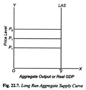
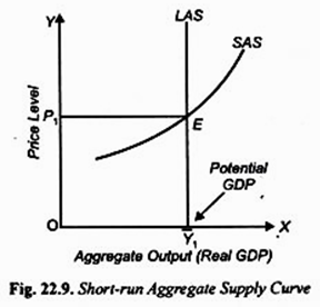
The long-run aggregate supply describes the relationship between the quantity of real GDP and the price level in the long run when real GDP equals potential GDP. The long-run aggregate supply curve is a vertical line (at potential GDP level as shown by LAS in Figure 22.7.

The long-run aggregate supply is vertical because potential GDP does not vary with price level, that is, it is independent of the price level. The reason for the independence of potential GDP from the price level is that the movement along the long-run aggregate supply curve involves not only the change in price level of goods but also prices of factor inputs such as wages of labour etc.

For example, when there is 5 per cent decrease in the prices of goods and services, this is matched by the same (i.e. 5 per cent) decline in wage rate and other factor prices so that relative prices and real wage rate remain unchanged. This explains why it is profitable to produce the same quantity of real GDP at lower price level of goods and services.

When price level of goods and services falls, the cost also falls as wage rate and other factor prices fall by the same percentage. Therefore, aggregate supply of output (i.e. real GDP) in the long run also remains constant at potential GDP level.

It is evident from above that long-run aggregate supply curve is the same as the classical aggregate supply curve.

Changes in Long-Run Aggregate Supply Curve:

Long-run aggregate supply curve is a vertical straight line at the level of potential GDP. Changes in price level bring about a movement along the long-run aggregate supply, but the quantity of aggregate supply remains fixed at the level of potential GDP. It is changes in potential GDP that causes a shift in the long-run aggregate supply curve.

The following factors cause a change in potential GDP resulting in a shift in the long-run aggregate supply curve:

1. The change in the full-employment quantity of labour.

2. Change in the stock of capital.

3. Progress in technology.

Increase in Labour Force:

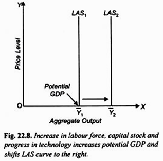
Labour is an important resource of production. Over time, given the capital stock and the state of technology potential GDP will increase as full-employment quantity of labour force increases. Therefore, the increase in the full-employment quantity of labour force causes a shift in the long-run aggregate supply curve to the right as shown in Figure 22.8.

It may be noted that changes in labour employment over the business cycle cause fluctuations in real GDP. But these changes in real GDP that take place over the business cycle are not changes in potential GDP. Changes in potential GDP occur due to changes in labour force and stock of capital, and improvement in technology.

Growth in the Stock of Capital:

The stock of capital in an economy determines the productive capacity of the economy. The larger the stock of capital in the economy, the more productive is the labour force of the economy and the greater is its potential GDP. The higher per capita output and potential GDP of the American economy as compared to those of the Indian economy are mainly due to the greater stock of capital in the United States.

Note that in the capital stock the modern economists include not only physical capital but also human capital. Human capital means the acquired skills, education and training of the workers. Like the increase in labour force, growth in capital stock also brings about increase in potential GDP and causes a shift in the long-run aggregate supply curve (LAS) to the right.

Progress in Technology:

Progress in technology enables firms to produce more from the given resources. Empirical research studies have shown that technological progress is by far the most important source of increase in GDP over the past two centuries. It is due to advances in technology that a modern worker, both in industry and agriculture, produces many times more output than the worker in the olden times. Thus, even with the fixed quantities of labour and capital, progress in technology raises potential GDP and causes shift in the long-run aggregate supply curve to the right.

We have shown long-run aggregate supply curve LAS and short-run aggregate supply curve together in Fig. 22.9. It will be seen that short-run aggregate supply curve at potential GDP level and beyond potential GDP level Y₁, it becomes highly steep.

Determination of GDP and Price Level: As-Ad Model:

Having explained the concepts of aggregate demand and aggregate supply with variable price level, now we shall explain how macroeconomic equilibrium is reached between the aggregate supply and aggregate demand to determine the amount of real GDP and the price level.

As there is difference between the long-run and the short run aggregate supply curves, the long-run equilibrium differs from the short-run macroeconomic equilibrium. While long-run equilibrium is the state towards which the economy is moving, short-run equilibrium is the actual state of the economy in the short run as it fluctuates around potential GDP.

The purpose of AS-AD model is to explain how the changes in various factors, fiscal and monetary policies bring about changes in real GDP and the general price level, that is, inflation. We explain below both the short-run and long-run macroeconomic equilibrium.

Short-run Macroeconomic Equilibrium:

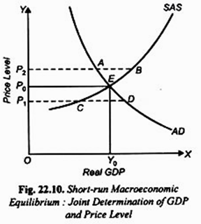
Short-run macroeconomic equilibrium occurs at the price level at which aggregate output demanded equals aggregate supply of output. That is, short-run equilibrium is reached at the price level at which aggregate demand curve AD intersects the short-run aggregate supply curve SAS.

This is shown in Fig. 22.10 where AD is the aggregate demand curve and SAS is the short-run aggregate supply curve. It will be seen that the short-run macroeconomic equilibrium occurs at point E at which the price level is P₀ and the real GDP is Y₀.

If price level is different from P₀, the economy will not be in equilibrium. Suppose, for example, price level is P₂, the quantity P₂A of the real GDP demanded at P₂ is less than the quantity P₂ B of real GDP supplied. This means the firms will not be able to sell all their output.

As a result, unintended inventories well pile up and firms will cut both production and prices. The process of cutting production and prices will continue until the equilibrium price level P_Q is reached and real GDP produced and sold is Y₀.

Now suppose that price level is P₁. It will be seen from Fig. 22.10 that at price level P₁ the quantity of aggregate output demanded (P₁D) exceeds the aggregate supply (P₁C). Thus at the price level P₁, the people will not be able to get all the goods and resources they want to buy.

As a result, inventories of goods with the firms will decrease below the desired level. This will induce firms to increase production and raise prices. The production and price level will rise until price level P₀ is reached and real GDP produced is Y₀ which meets the demands of the people fully at the price level P₀. Thus, the price level P₀ and real GDP equal to Y₀ represent the short-run macroeconomic equilibrium.

It is worthwhile to note that in the short run the money wage rate is fixed. It does not adjust to bring macro-equilibrium at full-employment level of real GDP. Thus, in the short run macro- equilibrium can be attained with real GDP less than or greater than potential GDP (i.e. the level of GDP at which there is full employment of labour) depending on the level of aggregate demand. It is only in the long run when money wage rate adjusts that equilibrium is restored at potential GDP.

It is worth noting that, as Keynes emphasized, the equilibrium between aggregate demand and aggregate supply may not necessarily be at full-employment level. Besides, when the economy is working at the level of full productive capacity, the increase in aggregate demand will lead to inflation in the economy.

Shift in Short-run Aggregate Supply Curve and Stagflation:

Let us now turn to examine the effect of changes in aggregate supply, aggregate demand remaining constant. With the advent of supply-side economics and new classical macroeconomics embodying rational expectations in recent years economists are increasingly concerned with shifts in aggregate supply curve.

Important factors that cause a shift in supply are changes in factor-prices and availability of resources, change in productivity and expectations about future inflation. Institutional factors such as Government regulations that affect resource use efficiency also cause shift in aggregate supply curve.

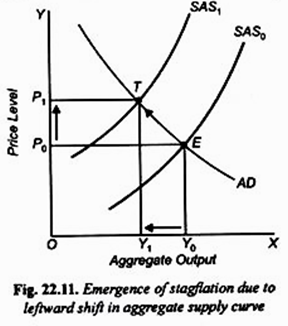
An important cause of shift in aggregate supply curve is the rise in prices of resources such as large increase in oil price by OPEC in 1973-74 and again in 1979-80. The rise in oil prices causes the aggregate supply curve to shift to the left as shown in Figure 22.11 where due to the higher per unit resource cost aggregate supply curve has shifted leftward from SAS₀ to SAS₁.

The aggregate demand curve AD remaining constant, with the leftward shift in aggregate supply curve from AS₀ to AS₁ leads to the new macroeconomic equilibrium being established at T, at which price level is higher and aggregate output smaller than before.

The emergence of rise in price level or inflation due to the leftward shift in aggregate supply curve is called cost-push inflation. There is an important difference between demand-pull inflation cost-push inflation. Whereas in case of demand-pull inflation, price rises along with rise in GDP, in case of cost-push inflation price level rises but GDP declines.

Thus, in Fig. 22.11 leftward shift in the SAS curve leads to rise in the price level from P₀ to while national output falls from Y₀ to Y₁. When both inflation and recession occur simultaneously, economists call this situation as stagflation. We thus see that increase in costs or resource prices are both inflationary and recessionary.

It may be noted that stagflation is also said to occur when instead of absolute fall in aggregate output there is slowdown in economic growth rate when inflation rate remains steadily high and also unemployment levels are quite high. It is evident from above that stagflation occurs as a result of supply shock, that is, rise in price of essential inputs such as crude oil which causes a shift in the short-run aggregate supply curve to the left.

Given the aggregate demand curve, the new equilibrium is reached at a higher price level (i.e., inflation) and at the same time reduced aggregate output (i.e., GDP) which generates unemployment in the economy.

We have explained above stagflation as a result of sharp rise in price of crude oil effected by restriction of oil output by collusive agreement of OPEC. In India stagflation can arise when there is decline in agricultural output due to failure of monsoon.

The decline in agricultural output causes food inflation which in turn leads to rise in wages of workers which causes a shift in the short-run aggregate supply curve to the left. Besides, drastic decline in agricultural output also leads to the rise in prices of raw materials provided by agricultural sector to industries. The rise in raw material prices for industries shifts aggregate supply curve to the left causing both inflation and reduction in output.

Solution:

To solve the problem of stagflation is a difficult task. In the seventies when the problem of stagflation was first faced efforts were made to solve it through demand management policies. However, when to reduce inflation, steps were taken to reduce aggregate demand by cutting expenditure, the result was decline in aggregate output which further worsened the unemployment problem.

On the other hand, when to reduce unemployment attempt was made to increase aggregate expenditure through expansionary fiscal and monetary policies, the result was acceleration in inflation.

The proper solution of stagflation is to shift the short-run aggregate supply curve to the right by reducing cost through raising productivity levels. The productivity in both industry and agriculture can be raised through technological improvements and more capital accumulation.

Besides, rightward shift in short-run aggregate supply can be made by reducing indirect taxes such as excise duties, sales tax, customs duties not only on final products but also on essential inputs used in the production of commodities.

Role of Fiscal and Monetary Policies in Keynesian, Monetarist and Classical Models:

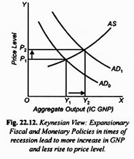
With this aggregate demand-aggregate supply model, popularly known as AD-AS model, we can explain the effects of fiscal and monetary policies on aggregate output (i.e., GNP) and price level in the economy. For example, if Government steps up its expenditure without increasing taxes, this will cause aggregate demand curve AD to shift to the right and thereby will lead to the increase in Gross National Product (i.e., National Income) and the price level as is illustrated in Figure 22.12.

Likewise, expansion in money supply, increase in private investment, or reduction in taxes without reducing Government expenditure will also result in shift in the aggregate demand curve to the right causing price level and national output to increase.

An important result follows from this AD-AS model. With flexible prices when under the influence of expansionary policies aggregate demand curve shifts to the right. To what extent it will affect the national output and the price level depends on the elasticity of aggregate supply curve.

Keynesian economists i.e., followers of Keynes are of the view that the aggregate supply curve is relatively elastic (i.e., flat), especially in times of recession, and therefore most of the response to expansion in aggregate demand will be the increase in output rather than rise in the price level as is shown in Figure 22.12.

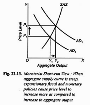
On the other hand, monetarists think that the supply curve is steep as is shown in Fig. 22.13 and in this case the expansionary fiscal and monetary policies causing outward shift in AD curve will bring about rise in price more than the increase in output.

In the extreme case of perfectly elastic aggregate supply curve which Keynes assumed in his analysis of depression increase in aggregate demand will not affect the price level and its full effect will be to raise the level of GDP.

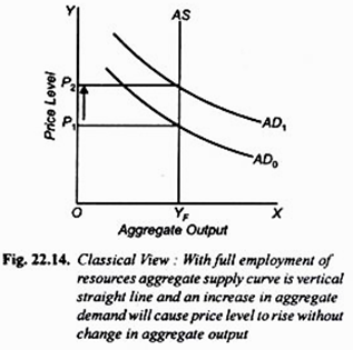
Lastly, when the economy is operating at the level of capacity output (i.e., full employment level) as the classical economists assumed, increase in aggregate demand in this case will lead only to higher price level or inflation in the economy without affecting aggregate output (national income).

The view of classical economists is illustrated in Figure 22.14 where aggregate supply curve AS is a vertical straight line at the full-employment level of output OY_F. It will be seen from this figure that when as a result of expansionary fiscal and monetary policies aggregate demand curve shifts outward to the right from AD₀ toAD₁, price level rises from P₁ to P₂ whereas aggregate output remains constant at OY_F level.