Aggregate Demand Curve: A Close View

The below mentioned article provides a close view on aggregate demand curve. Aggregate demand is the relationship between then quantity of output and the aggregate price level.

The Quantity Equation as Aggregate Demand:

The quantity theory tells us that, MV = PY. where M is the money supply, V is the velocity of money (which is assumed constant), P is the price level, and Y is the amount of total output.

This equation states that the money supply determines the nominal value of output which is PY.

We know that the quantity equation can be written in terms of the demand for and the supply of real money balances:

(M/P)^s = (M/P)^d = ky where k = 1/v.

Now the quantity equation states that the supply of real balances (M/P)^s equals the demand (M/P)^d and that the demand is proportional to the amount of output, Y.

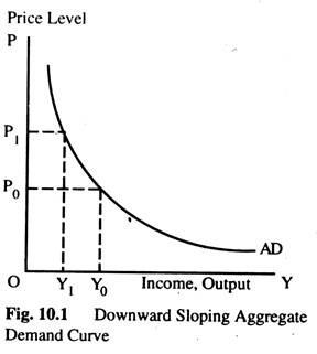
For any fixed money supply, the quantity equation shows a negative relationship between the price level P and output Y as in Fig. 10.1. This is called the Aggregate Demand Curve (ADC).

Why Aggregate Demand Curve Slopes Downward?

The aggregate demand curve slopes downward because for any fixed money supply, the quantity equation fixes the nominal value of output PY. Thus, if the price level goes down, output must go up and vice versa.

Better way to understand negative relationship between P and Y is to consider the link between money and transactions. Since we have assumed that V is constant, the money supply determines the money value of all transactions in the economy. If the price level falls, so that each transaction requires less money, the quantity of transactions and, thus, the quantity of goods and services purchased, must rise.

We could also look at the demand and supply of real balances. If Y is higher, people engage in more transactions and need higher real balances M/P. For a fixed money supply M. higher real balances imply a lower price level. Conversely, if the price level is lower, real money balances arc higher; the higher real balances allow a greater volume of transactions and, thus, a higher level of Y.

Shifts in the ADC (Aggregate Demand Curve):

The ADC is drawn on the assumption of fixed money supply. In other words, it tells us the possible combinations of P and Y for a given value of money supply (M^s). If the money supply changes, the possible combinations of P and Y change — that is, the ADC shifts. Let us examine the situations in which a shift may occur.

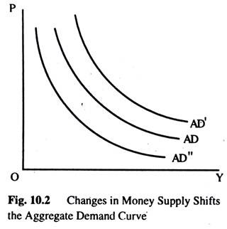
First, consider what happens when monetary authority increases the money supply. The quantity equation, MV = PY, tells us that there is an increase in PY. For any given output, the price level is higher, for any given price level, the output is higher Fig. 10.2 shows the ADC shifts outward to AD”.

Next, consider what happens when the monetary authority reduces the money supply. The quantity equation, MV = PY, tells us that the reduction in the money supply leads to a proportionate reduction in the nominal value of output, PY. For any price level, the amount of output is lower, and for any given output, the P level is lower. Fig. 10.2 shows the ADC curve shifts inward to AD”.

Aggregate Supply Curve (ASC):

The ADC, by itself, does not tell us about the price or output; it merely gives a relationship between these two variables. We need another relationship between P and Y that accompany ADC — an ASC. The ADC and the ASC together give us the equilibrium price level and output.

Aggregate Supply is the relationship between the quantity of goods and services supplied and the price level. Because prices are flexible in the long run and fixed in the short run, we need to discuss two different AS curves, the long run ASC (LRASC) and the short run ASC (SRASC) and the transition from the Short Run to the Long Run Aggregate Supply Curve.

The Vertical ASC in the Long Run:

We derive the long run ASC from the classical model. We know that the amount of output produced depends on the amounts of Capital and Labour and on the available technology.

To show this, we write:

Y = F (K₀, L) = Y

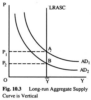
According to the classical model, output does not depend on the price level. Thus, the LRASC is vertical as in Fig. 10.3. The intersection of the ADC with this vertical LRASC determines the price level.

If the LRASC is vertical, then changes in ADC affect prices but not output. For example, if the money supply falls, the ADC shifts downward, as AD₂ in Fig. 10.3. The economy moves from A to B. This shift in AD affects only prices.

The vertical LRASC satisfies the classical dichotomy, since it implies that the level of output is independent of the money supply. This long-run output level, Y, is called the full-employment or natural level of output. It is the full-employment level of output or, more realistically, at which unem­ployment is at its natural rate.

The Short Run Aggregate Supply Curve (SRASC):

The vertical ASC or the classical model apply only in the long run. In the short run, some prices are sticky and, thus, do not adjust to changes in demand. This price stickiness implies that the SRASC is not vertical.

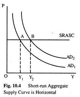
As an extreme case, all prices are fixed at predetermined levels. At these prices, firms are willing to sell as much as they could, and they hire just enough labour to produce the amount demanded. Since the price level is fixed, we represent this situation in Fig. 10.4 with a horizontal ASC.

The short-run equilibrium of the economy is the intersection of the ADC and this horizontal SRASC. In this case, changes in AD do affect the level of output. For example, if the monetary authority suddenly increases the money supply, the ADC shifts outward as in Fig. 10.4. The economy moves from the old intersection of AD and AS at point A, to the new intersection at B.

Since the price level is fixed, the shift in AD causes output to rise as in Fig. 10.4. A rise in AD increases output in the short-run because prices do not adjust instantly. After a sudden rise in AD, firms are stuck with prices that are too low. With demand high and prices low, firms sell more of their product, which causes them to increase employment and production.

From the Short-Run to the Long Run:

We can summarize our analysis so far as follows:

Over short periods of time, prices are sticky, the SRASC is fiat, and changes in AD affect the output of the economy over the long period of time, prices are flexible, the LRASC is vertical, and changes in AD affect only the price level. Thus, changes in AD have different effects over different time period.

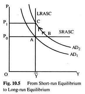
Let us trace the effects over time of a rise in AD. Suppose the economy begins in long-run equilibrium, as shown in Fig. 10.5 where there are three curves: the ADC, the LRASC, and the SRASC. The long-run equilibrium is at the point where ADC cuts the LRASC. Prices have adjusted to reach this equilibrium. Thus, when the economy is in its long-run equilibrium, the SRASC must cross at this point as well.

Now, suppose that the monetary authority increases the money supply. In the short-run prices are sticky, so the economy move from point A to B. Output and employment increases above their natural levels, which means the economy is in boom. Overtime, in response to the high demand, wages and prices rise. The gradual increase in the price level moves the economy upward along the ADC to point C, which is the new long-run equilibrium. In the new equilibrium (C), output and employment are back again to their natural levels, but prices are now higher — (P₁) than the (P₀). old price level long-run equilibrium point A.

Shocks and Instability:

Shocks disrupt economic well-being by pushing output and employment away from their natural rates. The model of AD and AS shows how shocks cause economic fluctuations.

The model is also useful for evaluating how macroeconomic policy car: respond to shocks in order to dampen fluctuations. Stabilization policy is public policy aimed at keeping output and employment at their natural rates.

Shocks to AD:

Suppose the invention of automatic teller machines reduced money demand by half. This fall in money demand is equivalent to an increase in the velocity of money. We know that (M/P)^d = ky where k = 1/v. A decrease in real money balances for any amount of output implies a decrease in k and an increase in V. Because people hold fewer money in their hands, the money circulate more quickly. Hence, velocity increases.

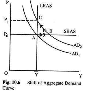
If the money supply is held constant, the increase in velocity causes nominal spending to rise and the ADC to shift upward, as in Fig. 10.6. In the short- run, the increase in demand raises the output — thus, it causes an economic boom. At the existing prices, firms sell more. The econo­my begins in long-run equilibrium, at A. An increase in AD — due to an increase in the velocity of money moves the economy from A to B, where output is above the natural (potential) level.

Over time, the higher level of AD increases wages and prices. As the price level rises, the quantity of output demanded declines, and the economy gradually approaches the natural rate of production, and the economy moves from B to C. But during the transaction, the economy’s output is higher than the natural rate.

What can the monetary authority do to dampen this boom? It might reduce the money supply to offset the increase in velocity which would stabilize AD’. Thus, the monetary authority can reduce or even eliminate the impact of demand shocks if it can control the money supply.

Shocks to AS:

A supply shock is a shock to the economy that alters the cost of production and, as a result, the prices that firms charge. Supply shocks have a direct impact on the price level; they are also called price shocks.

Examples are:

(1) A drought that destroys crops,

(2) A new environment protection law,

(3) The OPEC cartel and

(4) An increase in Union aggressiveness.

All these are adverse supply shocks; they push up costs and prices. A favourable supply shock reduces costs and prices.

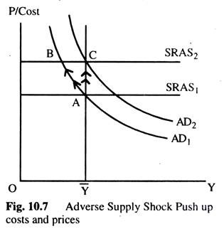
Fig. 10.7 shows how an adverse supply shock push up costs and prices. The SRASC shifts upward. If AD is held constant, the economy moves from A to B, leading to a combination of increasing prices and falling output below the natural rate. An experience like this called stagflation, because it combines stagnation with inflation. Eventually, as prices fall, the economy returns to the natural rate at A. But the cost of this process is a painful recession.

In response to an adverse supply shock, the policy maker can increase AD to prevent a reduction in output. If the increase in AD coincides with the shock to AS, the economy moves immediately from point A to C as in Fig. 10.7. In this case, the monetary authority is said to have accommodated” the supply shock. The cost of this policy is permanently higher level of prices. There is no way to adjust AD — both to maintain full employment and to keep the price level stable.

The IS-LM Model and the Theory of Aggregate Demand Curve:

We used the IS-LM model to explain national income in the short-run when the price level is fixed. To see how the IS-LM Model fits into the model of AD and AS developed above, we now examine what happens in the IS-LM model as the price level changes. The IS-LM model provides a theory to explain the position and slope of the ADC.

As we have seen, the ADC is a relationship between the price level and the level of national income. We derived this relationship from the quantity theory of money. For a given money supply, a higher price level implies a lower level of income (Y). Increase in the money supply shift the ADC outward, and decrease in the money supply shift the ADC inward.

We now use the IS-LM model to derive the ADC. First, we use the IS-LM model to show that national income falls as the price level rises; the downward sloping ADC expresses this relationship. Second, we examine what causes the ADC to shift.

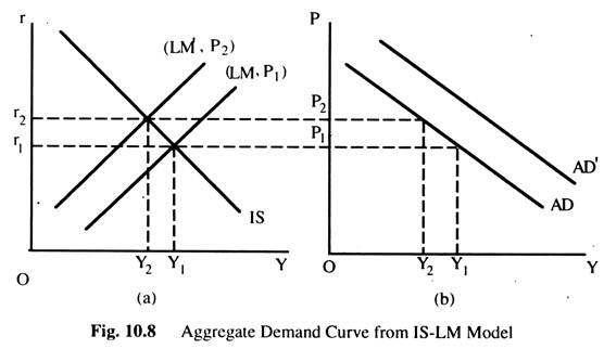
The ADC is downward sloping because in a given nominal money supply increase in price level causes a lower supply of real balance (M/P). A lower supply of real balances shift the LMC upward, which raises the interest rate and lowers equilibrium level of income, as in Fig. 10.8(a). We can see that when the price level rises from P₁ to P₂, national income tails from Y₁ to Y₂. The ADC in Fig. 10.8(b) plots the negative relationship between national income and the price level that arises from IS-LM model.

What causes the ADC to shift?

Because the ADC summarizes the results of the IS-LM Model, shocks that shifts the ISC or the LMC cause the ADC to shift. Expansionary fiscal or monetary policy raises income in the IS-LM model and thus shifts the ADC outward as in Fig. 10.8(b). Similarly, contractionary fiscal or monetary policy lowers income and thus shifts the ADC inward.

To sum up, a change in income in the IS-LM model resulting from a change in the price level represents a movement along the ADC. A change in income in the IS-LM model resulting from a change in fiscal or monetary policy for a fixed price level it represents a shift in the ADC.

Monetary and Fiscal Policy Change Shift the ADC: Monetary Policy Change:

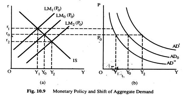
Fig. 10.9(a) shows a monetary policy change. For any given price level,, an increase in the money supply raises real money balances, shifts the LMC downwards and raises Y ; and a decrease in the money supply decreases real money balances, shifts the LMC upward, and lowers income. Thus, an increase in money supply shifts the ADC to the right to AD’ and a decrease in money supply shifts it to the left to AD” from AD₀ as Fig 10.9(b) shows.

Fiscal Policy Change:

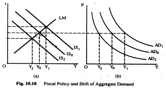
Fig 10.10(a) shows a fiscal policy change — a fiscal expansion, such as an increase in government expenditure or a decrease in taxes; a fiscal contraction, such as decrease in government expenditure or an increase in taxes. The fiscal expansion shifts the ISC outward or fiscal contraction shifts ISC inward and, for any given price level, raises or reduces income. Hence a fiscal expansion shifts the ADC outward from AD to AD₁ or a fiscal contraction shifts the ADC inward from AD₀ to AD₂ as Fig. 10.10(b) shows.

The IS-LM Model in the Short-Run and Long-Run:

The IS-LM model is designed to explain the economy in the short-run when the price level is fixed. Now we know how a change in the price level influences the equilibrium, we can also use the IS-LM model to describe the economy in the long run when the price level adjusts to ensure that the economy produces at its natural rate. By using the IS-LM model to describe the long-run, we can show clearly the difference between the Keynesian and the Classical Model.

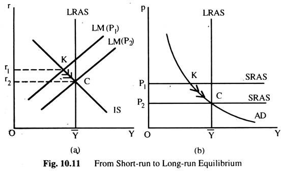
Fig 10.11(a) shows the three curves — the IS , the LM and the LRASC representing the natural rate of output Y — that are necessary to understand the short-run and long-run equilibrium The LMC is drawn for a fixed price level (here it is P₁). The short-run equilibrium of the economy is point K, where the ISC intersect the LMC.

Fig. 10.11(b) shows the same situation in the diagram of AD and AS. At the price level P₁, the quantity of output demanded is below the natural rate In other words, at the existing price level, there is insufficient demand for goods and services to keep the economy at its full employment level.

In Fig. 10.11(b) we examine the short-run equilibrium at which the economy finds itself and the long-run equilibrium towards which the economy moves Point K describes the short-run equilibrium, where it is assumed that price level is fixed (P₁). Eventually, the low demand for output causes the price to fall, which moves the economy back towards its full employment level (natural rate).

When the price level reaches P₂, the economy is at point C, which is the long-run equilibrium. In Fig. 10.11(b), AD = AS at point C, and the quantity of commodity demanded equals the natural rate of output Y. This long-run equilibrium is reached in Fig. 10.11(a) in the IS-LM Model by a shift in the LMC. The fall in price level (P₁ to P₂) increases real money balances and thus shifts the LMC to the right to intersect with the ISC at C.

We can now see the difference between Keynesian and Classical approaches to the determination of national income and employment. The Keynesian assumption is that the prices and wages are fixed at point K. Depending on monetary, fiscal and other determinants of AD, output and employment may deviate from the natural rate.

The classical assumption is that prices and wages are flexible and eventually reached at point C. The prices and wages adjust to ensure that national income and employment are always at the natural or full employment level.

In other words, we can think of the economy as being described by three equations. The first two are the IS and LM equations,

(1) Y = S(Y) + l(r)                                     (IS)

(2) M = L(r, Y) = kPY +L(r)                   (LM)

These two equations — IS and LM — contain three variables: Y, r and P. The classical approach is to complete the model with the assumption that output reaches the natural rate, so the third equation is (3) Y = Y. This assumption implies that r and P must adjust to satisfy the IS and LM equations.

The Keynesian approach is to complete the model with the assumption of fixed prices, so the third equation is (3′) P = P₁. This assumption implies that, r and Y must adjust to satisfy the IS and LM equation.

What assumption is most appropriate? The answer depends on the time horizon. The classical assumption best describes the long run. The Keynesian assumption best describes the short-run.

General Equilibrium with Flexible Wages:

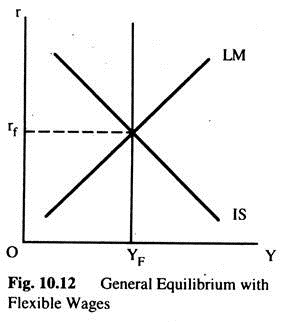
In Fig. 10.12 the IS and LM curves summarize the conditions of equilibrium in the goods and money sectors, respectively. The Y_F line shows the one level of output at which the labour market is in equilibrium — the quantity of labour demanded is equal to the quantity of labour supplied.

The Y_F is vertical because, on our present assumptions, the interest rate plays no role in the determination of equilibrium in the employment sector. Any point off the Y_F line implies an excess demand or an excess supply of labour, which will lead to change in the real wage rate, employment and output. For the entire economy to be in equilibrium we must have equilibrium in all sectors.

If any sector is not in equilibrium, some variables in that sector must change and this is likely to affect the combination of real income and interest rate at which all three sectors are in equilibrium — AD is equal to total output; the quantity of money demanded is equal to quantity of money supplied and the quantity of labour demanded is equal to the quantity of labour supplied.

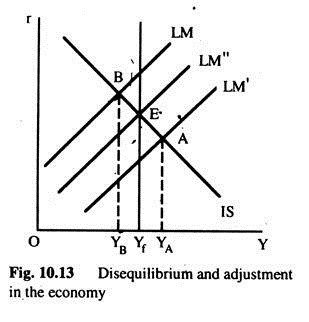
To have a better understanding about the equilibrium, we will examine the forces generated in the system in disequilibrium, and how these forces operate to bring the economy back to equilibrium. In Fig. 10.13 two possible disequilibria are shown.

With the IS curve and LM’ curve, the money and goods sectors are in equilibrium at point A where the AD is at Y_A. However, given the condition in the employment sector, and the production function, actual output is Y_f. There is thus excess demand for goods and services equal to Y_A-Y_f. Given our present assumptions about the effects of this discrepancy, the disequilibrium at point A will lead to a rise in prices.

We can now use our analysis to see how this rise in prices will affect some or all of the variables entering the determination of equilibrium in the goods and money sectors, and whether the price rise will tend to eliminate the disequilibrium.

We have seen that changes in the price level have no effect on any of the variables used in the construction of IS curve. We assumed that the behaviour represented by the IS curve (C + I) is not affected by the price level — it is all expressed in real terms. However, we know that changes in the price level do affect equilibrium in the money sector, though the demand for money is specified in real terms, the supply of money is given in nominal terms.

Thus, the rise in the price level generated by the excess of desired expenditure over output will lead to a leftward shift of LM curve. The rise in prices will continue as long as there is an excess of AD over output (Y_A > Y_f), which means as long as the IS and LM curves intersect to the right of E.

When the real quantity of money is such that LM’ coincides with LM” curve, all the sectors would be in equilibrium again. The change in the price level eliminates the discrepancy between desired expenditure and Y_F (Y_A ≠ Y_F) by changing AD. However, this does not occur directly. The change in the price level has a direct effect on the real quantity of money.

The change in AD occurs because of the link between the real quantity of money and the interest rate and also because of the link between the interest rate and investment. These links are implicit in the IS and LM model.

It should however be noted that the change in the price level has no effect on Y_f curve, which shows equilibrium in the employment sector, because all the behavioural variables in that sector were specified in real terms. It is true that, given any money wage rate, a change in the price level will affect the real wage rate, but on our present assumptions any change in the real wage, due to a change in the price level, will be offset by a change in the money wage rate, as we have seen before. Only’ at the real wage rate the labour market is in equilibrium.

Let us now examine the disequilibrium at point B in Fig. 10.13. At point B, AD = Y_B. If the employment sector is in equilibrium, output is equal to Y_f, and at point B output is greater than AD (Y_f > Y_B). This will reduce prices and increase the real quantity of money (LM curve shifts towards LM”), which will result in a fall in the interest rate and, thus, arise in desired investment. This process will continue so long as output is greater than AD and a new equilibrium is reached at E.

Another possibility is that at point B the goods sector is in equilibrium, AD = Y_B output, but the employment sector is not. There is, thus, no pressure on the price level. However, if the employment sector is not in equilibrium, something must change there. What sort of disequilibrium is implied by this situation? It might be an equilibrium at less than full-employment output, this situation implies an excess supply of labour. But this is not correct.

All we know is that, at B, employment is less than the full-employment. This may be either because the real wage rate is too high and there is an excess supply of labour or because the real wage rate is too low and there is an excess demand for labour. The employment sector is such that the wage rate will fall if there is an excess supply of labour and rise if there is an excess demand for labour.

In both cases, employment and output will rise. However, as output increases, a discrepancy would appear between AD and output; prices will start falling, the real quantity of money will start rising and AD will start rising, too. This process will continue until we have equilibrium in all sectors at E.

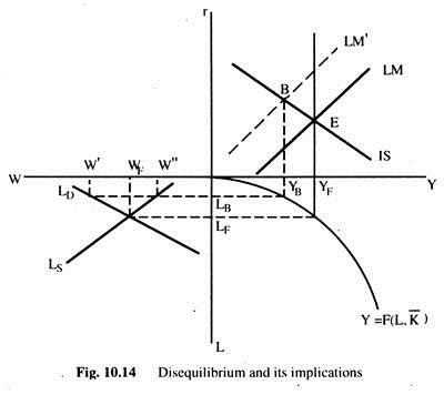
In Fig. 10.14 we can see the two possibilities just discussed and thus implications for the forces generated in the system. The top right quadrant gives all the sectors of the economy — the IS, LM and Y_F curves. The bottom right quadrant shows the production function relating output to employment, and the bottom left quadrant represents the labour market.

The two possible types of disequilibria represented by point B depends on whether employment at B is L_B or L_F. If employment is L_F the labour market is in equilibrium and output is Y_F. This means that — in the goods market — AD < Y_F. All prices fall, given the nominal stock of money, the real quantity of money rises, thus leading to a fall in the interest rate and rise in desired investment. This will shift the LM curve to the right and ultimately equilibrium will reach again in E. Real wages do not change— money wages change in the same proportion as the change in prices.

On the other hand, if employment is L_B and output would be Y_B the point B represents equilibrium in the goods market → AD =Y_B — but dis­equilibrium in the labour market. Either the real wage rate is too high (W’) and there is an excess supply of labour, or it is too low (W”) and there is an excess demand for labour.

In the former case, the money wage rate will fall (and also real wage rate falls), and in the latter case it will rise. In both the cases employment and output will increase which will mean that equilibrium in the goods market no longer exists. Output (Y_F) > than AD and this leads to a fall in prices and an increase in AD. This process will continue until point E is reached where the economy will be in equilibrium again. Real wages change to equilibrate the labour market.

Thus, we can sec that the variables play a crucial role in equilibrating the whole system; the price level and the wage rate. Changes in the price level produce equilibrium in the goods sector, changes in the wage rate produce equilibrium in the employment sector.

It is clear from the above analysis that wages and prices have to be flexible to be effective in equilibrating the system. They have to react to disequilibrium — prices in the goods market, and wages- in the labour market. Moreover, the links by which changes in these two variables affect output (Y) and AD have to be operative.

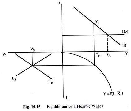
For example, if disequilibrium in the goods market affects the price level but condition in the money market is such that changes in the price level do not have any effect on the interest rate — and, thus, have no effect on desired investment — then the price level does not have any effect on output and AD. This situation will prevail where we assume that the supply of money is perfectly elastic and, thus, the LMC is perfectly elastic too as Fig. 10.15 shows.

With flexible wages, total output will always be Y_F; otherwise the wage rate will change. This situation can be seen in Fig. 10.15, where AD (Y_A) is greater than output (Y_F), therefore, prices will start rising as before. However, the rise in prices would not be able to eliminate disequilibrium because the price rise has no effect on the employment sector as the employment sector is in equilibrium and money wages change in the same proportion as the price level, and, thus, real wages remain unchanged and, therefore, output and employment remain unchanged.

The rise in prices has no effect on AD; the LMC and the interest rate remain unchanged. Thus we see that even though the disequilibrium in the goods market results in changes in the price level, these changes cannot remove the disequilibrium because the condition in the money market is such that the link between the price level and AD has been broken.

Fixed Money Wages:

So far we have considered labour market which is always at full employment equilibrium and, thus, equilibrium output depends only on the supply of labour and on technology. This assumption implies that the money wage rate can change when there is an excess supply or demand for labour. It is only via changes in the money wage rate that a disequilibrium in the employment sector affects the real wage rate.

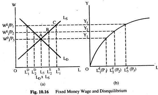
We now assume that the wage rate is not flexible in downward direction. We still assume that, the quantity of labour supplied is a function of real wage rate, but we add to this the assumption that, no labour will be supplied below some fixed money wage. With these assumptions, the labour market is shown in Fig. 10.16.

The vertical axis measures the real wage rate, for some fixed money wage rate W⁰ and various price levels, where P₁ <P₂ <P₃ and the horizontal axis measures the quantity of labour. The demand curve for labour is still a function of the real wage rate. But labour supply curve is now different at different price levels, because of the assumption that at any money wage below W⁰ no labour will be supplied. When the price level is P₁ the real wage rate would be W⁰/P₁. The maximum amount of labour supplied at the real wage W⁰/P₁ is L^S₁.

However, our assumption is that at any money wage below W⁰ no labour will be supplied. Given the price level P₁, this assumption means that at any real wage below W⁰/P₁ no labour will be supplied and the supply curve is now o W⁰/P₁ CL^S. Now, if the price level is P₂ > P₁, the maximum quantity of labour supplied will be L^S₂ at the same money wage rate w⁰. However, for the price level P₂, the supply curve of labour is O W⁰/P₂ BL^S because of our assumption that no labour will be supplied at a real wage rate below W⁰/P₂.

Similarly for other price levels and different minimum money wage rate, say W⁰.

Let us now define equilibrium in a labour market in which the money wage rate is fixed. In Fig. 10.16(a), the real wage rate is W⁰/P₁ where W⁰ is the fixed money wage and the price level is P₁. At this real wage the quantity of labour demanded is L^D₁, the maximum quantity of labour supplied is L^s₁. There is, thus, an excess supply of labour.

However, given the assumption that the money wage is inflexible downwards, this excess supply of labour has no effect on the wage and, therefore, employment. For the given money wage W⁰ and price level P₁, the labour market is in equilibrium at L^D₁. Similarly, for the given money wage W⁰ and price level P₂, the labour market is in equilibrium at L^D₂. We can see that once a fixed money wage is introduced, employment becomes a function of the fixed money wage and the price level.

Fig 10.16(b) shows a production function relating output to employment for various price levels and the given fixed money wage W⁰. For example, when the price level is P₁, equilibrium employment is L^d₁, and the corresponding output is Y₁. Similarly for the other price levels.

Now there is no longer a single quantity of output corresponding to equilibrium in the labour market, but different outputs depending on the price level. The crucial difference between the previous model and the fixed wage model is that now the price level affects equilibrium employment and output.

General Equilibrium with a Fixed Money Wage:

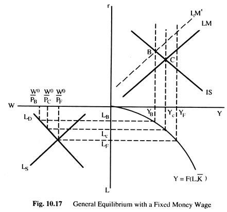
In Fig. 10.17 we combine the employment sector with fixed money wages and other sectors (money sector and goods sector). The top right quadrant gives all the sectors of the economy — the LM, IS and Y_F curves. The bottom right quadrant shows the production function relating output to employment, and the bottom left quadrant represents the labour market with the real wage rate which is now measured by W⁰/P, where W⁰ is the assumed fixed money wage.

Let us examine the situation at point B on the assumption that the LMC passing through this point represents equilibrium in the money sector for the price level P_B. Thus, AD at P_B equals Y_B. With the money wages fixed at W⁰ and the price level P_B, the real wage rate is equal to W⁰/P_B, and output and employment are equal to Y_B and L_B, respectively. Output is equal to AD and both the employment sector and the goods sector are in equilibrium; the excess supply of labour has no effect on employment and output and thus on the equilibrium.

Now we assume that the LMC passing through point B represents equilibrium in the money sector for the price level P_F and the fixed money wage W⁰. At the real wage rate of W⁰/P_F, employment is L_F and output is Y_F. The output is greater than AD. This (discrepancy will lead to a fall in prices, and an increase in the real quantity of money, a fall in the interest rate and thus an increase in AD (this will shift the LMC to the right).

However, the fall in prices also raises the real wage rate, and, thus, employment and output fall. This process will-continue as long as Y > AD; until point C is reached with the price level P_c. At this point, AD equals output at point Y_c, and all the sectors are again in equilibrium.

The main difference between the effects of the disequilibrium examined above and the identical disequili­brium examined under a flexible wage is that, there changes in prices were accompanied by changes in money wages, keeping the real wage rate and, thus, output, constant at the level associated with equilibrium in the labour market.

The Price Level:

The introduction of the employment sector into the model shows the importance of the price level in achieving overall equilibrium in the economy because of its effect on the AD and output (in flexible money wage it effects the AD only). Thus, it is important to understand exactly how the price level is determined, and what real variables are affected by it. Here we want to summarize the results.

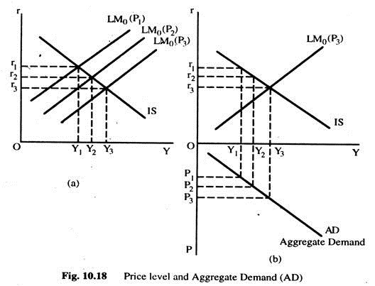
Fig. 10.18(a) shows various equilibria in the goods sector for a given IS curve, and a given quantity of nominal money M⁰ at various price levels P₁ > P₂ > P₃. We can see the relationship between the price level and AD. In the bottom half of Fig. 10.18(b) the relationship between the price level and AD is shown. This curve is drawn for the assumed conditions in the goods and the money sectors shown in Fig. 10.18(a). A shift in the IS curve or the supply curve of nominal money will shift the AD curve. The IS curve from Fig. 10.18(a) and LM curve for the price level P₃ are shown in the top half of Fig. 10.18(b).

We now turn to the relationship between the price level and aggregate supply (AS). We know already that whether AS depends on the price level or not, it depends on the conditions in the labour market, i.e. on whether the wage rate is flexible or not.

If the wage rate is flexible, employment is determined independently of the price level and thus AS is independent of the price level as well. If, however, the money wage is fixed, output and employment become a function of the price level. Fig. 10.19 shows these relationships.

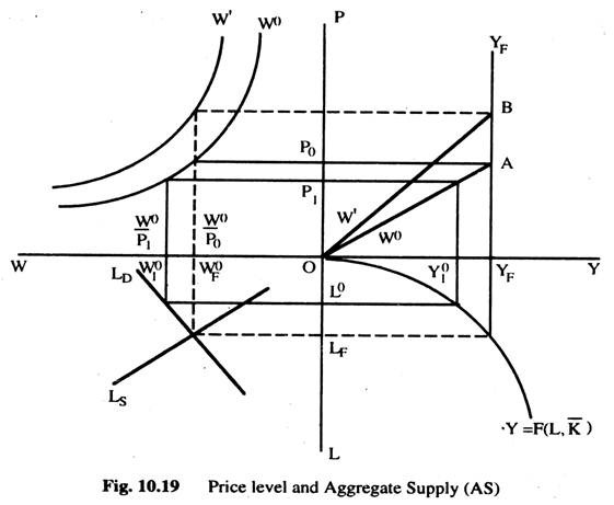
Fig. 10.19 represents the labour market (left quadrant) and the production function (right quadrant) in bottom two quadrants and the top left quadrant shows the relationship between the real wage rate (W⁰) and the price level (P) for some given money wage. Thus, W⁰ curve shows the relationship between the price level and the real wage (w = W⁰/P) when the money wage is fixed at W⁰.

Similarly, W’ curve, represents a money wage greater than W⁰. We derive the relationship between AS and the price level in the top right quadrant. If the money wage is flexible we can ignore the top left quadrant, because, in that case, the equilibrium real wage, employment and output are W_f, L_f and Y_f, respectively, whatever be the price level. With flexible money wages, AS is independent of the price level and is represented by Y_F Y_F.

Assume, however, that the money wage is fixed at W⁰. If the price level is P₀, the real wage rate is W⁰/P₀ < w_F, employment is L_F and output is Y_F. If the price level is P₁, the real wage rate W⁰/P₁ = W⁰₁, employment is L⁰, and output is Y⁰₁. If we do this for all price levels we get the curve W⁰AY_F showing the relationship between output and the price level. If the money wage is fixed at W’ > W⁰, the relationship between output and the price level is shown by the curve W’BY_F.

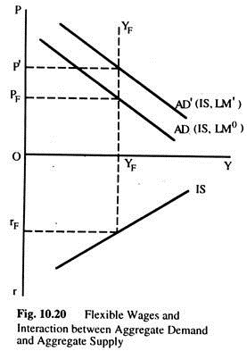
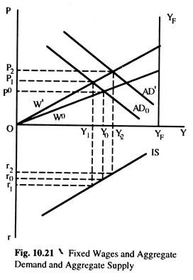
We can combine the AD curve from Fig.10.18 (b) and the AS curve of Fig. 10.19 to see the interaction between AD and output (AS). This is done in Fig. 10.20, for flexible wages and Fig. 10.21 for fixed wages. If wages are flexible the AS is represented by the Y_FY_F curve and Aggregate Demand by the AD curve, for the IS curve shown and a quantity of nominal money M⁰. Equilibrium in the economy is at Y_F and P_F and r_F. At any price level above P_F, output (AS) will be greater than AD, driving prices down; at any price level below P_F it will be AD > AS (output), driving prices up.

If the quantity of money changes to M’ > M⁰, AD shifts to AD’, the new equilibrium will be at Y_F. r_F and P’. The only effect of the change in the quantity of money is to change the equilibrium price level; nothing else is affected. The equilibrium interest rate and Fare determined independently of what happened in the money sector. For any given behaviour with respect to consumption and investment (i.e., for any given IS curve) the money sector (given by the LMC) only affects the price level.

The result seems strange, because when we analysed the money sector we saw that the interest rate was the equilibrating variable, reacting to any excess demand or supply of money, yet, when we put together the money sector with the rest of the economy, we find that the equilibrium interest rate is not affected by what happens in the money sector.

This seeming paradox is not hard to explain. Once we introduce an independent determinant of output, an employment sector with flexible wages, and assume that prices are flexible, the price level will always react to a disequilibrium between AD and AS (output) via its effects on the real quantity of money, thus, on the interest and on AD.

If the interest rate is not at that level which equates AD and output (AS), then price level will change, thus changing the interest rate. Only one interest rate (r_F) is compatible with equilibrium between AD and the given level of output and this interest rate will be achieved by changes in the price level.

Thus, starting from equilibrium, for example, Y_F, r_F and P_F, any change in the money sector will initially affect the interest rate as before, but this will have repercussions on the price level via the effect of the interest rate on AD, and this will offset the initial effect on the interest rate.

Thus far we have seen the price level in a situation in which wages are flexible and, therefore, output (AS) is independent of the price level. If money wage is fixed at W⁰, as in Fig. 10.21, the (AS) output curve is W⁰Y_F. With the AD curve AD₀, general equilibrium will be Y₀, P₀ and r₀.

At any price level above P₀, output (AS) will be greater than AD and prices will fall, increasing AD via its effect on the interest rate, and decreasing output (AS) via the effect on the wage rate; the opposite will occur at any price level below P₀. If the fixed money wage is W’, the new equilibrium will be one with a lower real income, a higher price level and a higher interest rate (Y₁, P₁, r₁).

Thus, all the factors that were relevant in determining the price level, we now have a new factor — the fixed money wage which affects output and the price level by interaction between output (AS) and AD. A change in the money sector, for example, an increase in the quantity of money from M⁰ to M’ will shift the ADC from AD⁰ to AD¹. The effect of this will be to raise income to Y₂ the price level to P₂, and to lower the interest rate to r₂.

Thus, change in the money sector do affect the interest rate and the price level. The difference between the present case fixed money wage and the previous one with flexible wages is that the initial effect of the change in the money sector of increased AD, and, thus, the price level, is accompanied by a change in output. Thus, the disequilibrium created between output (Y) and AD is eliminated both by a decrease in AD and increase in output (Y) due to rise in prices; in the previous case only the former occurred.

The Extreme Cases:

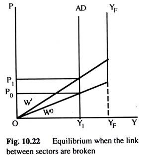
The above analysis can be used to examine the effects on equilibrium when the links between the monetary sector and the goods sector are broken, cither because the LM curve is perfectly elastic or because the IS curve is perfectly inelastic. Both of these would lead to a perfectly inelastic ADC Figure 10.22 shows a situation in which the money sector is characterised by a perfectly elastic LMC.

This is the top part of Fig. 10.21. First, let us assume that the employment sector is one with flexible wages; therefore, the Y_FY_F curve is the one representing the output sector. With the aggregate demand curve as AD, we see that AD at any price level are Y₁ and output at any price level is Y_F.

Because Y_F > AD, prices will fall but with our present assumptions this has no effect on any of the variables in the system. There is no way to achieve equilibrium in the system. If the AD curve cuts the Y axis to the right of Y_FY_F curve, prices would start rising and continue to do so without any effect on the system.

If the employment sector is characterized by the fixed money wage W^O the AS is shown by the curve W^OY_F. With the aggregate demand curve, AD, equilibrium would be at price OP_O. At any price level above P^O output is greater than AD and prices fall, raising real wages and thus reducing employment and output. A rise of the fixed money wage to W’ would raise the price level to PI leaving the real wage rate, output and employment unchanged. This is the situation in which it has no effect on AD. If the AD curve intersects the Y axis to the right of the Y_FY_F curve we would have the same situation as in the case of flexible wages.

The price level would continue to rise indefinitely.