The Great Depression of Aggregate Demand (With Diagram)

Let us make an in-depth study of the Great Depression of Aggregate Demand.

One of the major defects of the classical model is that it failed to explain the Great depression of the 1930s.

The IS-LM model suggests a fairly acceptable explanation of depression on the basis of Keynesian spending hypothesis.

The depression occurred due to a sudden and exogeneous fall in aggregate demand for goods and services. This decline in spending led to a leftward shift of the IS curve.

One plausible explanation of spending crash was a sudden fall in consumption expen­diture. The Wall Street Crash of October 1929 reduced wealth and increased uncertainty about the future prospects of the U.S. economy. It made most people overcautious and induced them to save more and spend less. Thus under-consumption of the masses was the cause of U.S. downturn, as has been predicted by Karl Marx.

Another explanation was that the investment boom of the 1920s. There was overinvestment in housing in this period.

The sudden fall in demand for residential buildings initially led to sectoral recession and then to economy-wide depression because consumption and investment fell together.

Moreover the contractionary fiscal policy in the form of a rise in taxes and a cut in government expenditure also reduced aggregate spending and shifted to the IS curve to the left. This fiscal action was taken to reduce the budget deficit even in the midst of high employment.

All the above changes occurred simultaneously and conjointly led to drastic cut in spending.

Friedman’s Money Hypothesis:

According to Friedman’s money hypothesis the sharp decline in the money supply caused most severe downturns in U.S. economic history.

This sharp contraction in money supply shifted the LM curve to the left and caused real interest to fall. But it did not stimulate investment due to widespread business pessimism. The monetary contraction was responsible for the rise in the unemployment in early 1930s.

Deflation as a Stabiliser:

In terms of this chapter’s IS-LM model falling prices raise income. If M remains constant, but P falls, real money balance increases. This shifts the LM curve to the right. So Y rises.

The Pigou Effect:

Falling prices may expand income through another mechanism, called the Pigou effect. Since real money balances are a part of households’ wealth, as P falls and M/P increases consumers feel that they are richer than before. So they spend more. This increase in C leads to a rightward shift in the IS curve, leading to a rise in Y. The Pigou effect has been called by Don Patinkin the ‘real balance effect’.

The Destabilising Effect of Deflation:

Another group of economists put forward an exactly opposite view about the effect of declining prices. One such view is captured by the debt-deflation theory. This theory brings into focus the adverse (contractionary) effects of unexpected fall in the price level.

The theory can now be presented in a nutshell. Unanticipated changes in the price level redistribute wealth between debtors and creditors. During deflation debtors lose and creditors gain. So debtors spend much less and creditors spend a little more. The end result is a fall in spending, a shift of the IS curve to the left and a lower Y.

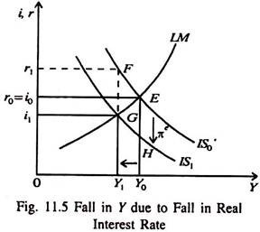
The basic debt-deflation mechanism is illustrated in Fig. 11.5. An expected (anticipated) deflation (indicated by the negative value of π^e) raises the real rate of interest (r) for any level of given nominal rate of interest (i).

This very fact pulls investment expenditure down and shifts the IS curve to the left (from IS₀ to IS₁). As a result income falls from Y₁ to Y₂. But here we find a surprising result. A fall in nominal interest rate from i₀ to i₁ and at the same time a rise in the real interest rate from r₀ to r₁.

Thus falling prices have a destabilising effect on the economy. In this modified IS- LM framework a fall in M can lead to a fall in Y, even if real money balances do not fall or even if nominal rate of interest rises.