Difference between Classicists and Keynes on Aggregate Demand and Aggregate Supply

This article will help you to learn about the difference between the Classicists and Keynes on Aggregate Demand (AD) and Aggregate Supply (AS).

Difference between Classicists and Keynes on Aggregate Demand and Aggregate Supply

The classical economists believed in the operation of the Say’s Law of Markets which states that supply creates its own demand. They also assumed sufficient wage-price flexibility. These two would automatically ensure full employment of resources in the classical macro-economy.

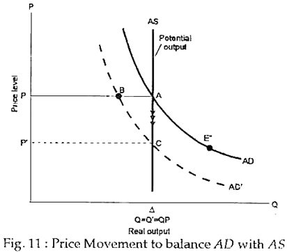
This point is illustrated in Fig. 11. The economy is at full employ­ment at point A and the price level is OP₁. Now, if the AD curve shifts downward due to any reason such as tight money or other external forces — from AD₁ to AD₂, the econ­omy initially moves to point B, which corresponds to the same price but lower output. But such a situation, according to classicists, would not per­sist for long.

A fall in demand and a consequent fall in output would lead to a fall in wages and prices. Thus, at the end of the process of adjustment, the general price level would fall from OP₁ to OP₂. With a fall in the general price level, actual output gradually returns to the full employment level is Q_F. Thus, the economy is enabled to re-achieve full employment (at a different point such as C instead of A).

Policy Consequences:

The classical view has two major consequences which are important from policy point of view. First, unemployment is a logical impossibility in the classical world. Unemployment, if any, will be of a temporary or frictional nature.

As A.C Pigou has pointed out:

“With perfectly free competition there will always be a strong tendency toward full employment. Such unemployment as exists at any time is due wholly to the frictional resistances [that] prevent the appropriate wage and price adjustments being made instantaneously”.

The second point to note here is that the government cannot alter the level of the employment and output through changes in policy variables. Instead, macroeconomic policies like stabilising monetary and fiscal policies can affect only the general price level and the composition of real GNP, as Fig.11 shows.

The Keynesian View of the Macro-Economy:

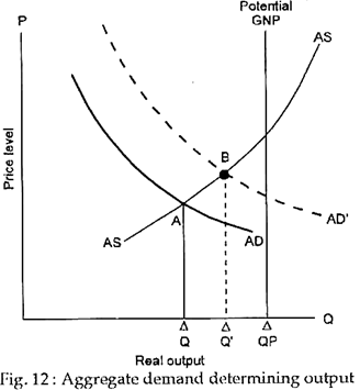
In the Keynesian model the AS curve slopes upward because Keynes was concerned with short-run problems of capitalism. Such a supply curve is shown in Fig. 12. This implies that so long as there are unemployed resources in the economy an increase in AD will lead to an increase in output or GNP, with no change in prices.

Keynes, in fact, assumed wage-price rigidity. When AD is low the economy will be in equilibrium at point A. But if AD in­creases from AD₁ to AD₂, the economy will reach equilibrium at point B, which corre­sponds to a higher level of output or GNP.

If AD falls output will fall and employment will also fall. Thus, un­employment is a logical possibility due to rigidity of wages and prices. And, it was Keynes who first introduced the concept of underemployment equi­librium — equilibrium at less (than) full employment. Point A or C in Fig. 12 illustrates such a situation where society’s actual output is less than it potential output.

As Samuelson and Nordhaus have put it “Keynes empha­sised that because wages and prices are inflexible there is no economic mechanism to restore full employment and ensure that the economy pro­duces its potential (output). A nation could remain in its low output, high-misery condition for a long time because there is no self-correcting mechanism or visible hand to guide the economy back to full employment.”

Policy Implications:

The Keynesian theory has an implication from the policy point of view. Since in the Keynesian model, the AS curve is upward sloping in the short run, economic policies (such as monetary and fiscal policies) that increase aggregate demand succeed in increasing output and employment, from Y₀ to Y₁ and Y_F, shown in Fig. 12. What about the policy implication of classical economics?

A few words may perhaps be spared about the policy implications of classical and Keynesian views of the macro-economy. Classical economists who believed in the Say’s Law of Markets were sceptical about the need for government action (in the form of remedial monetary and fiscal measures) to stabilise the economy (by controlling business cycles). They believed that a government policy aimed at increasing aggregate demand will instead lead to escalating inflation. But this is not the whole of story.

The classicists were also worried about the growth- constraining effect of government spending. They argued that government expenditure would always be at the expense of private investment. This is known as the crowding-out effect, which means that when the government increases its own expenditure (to increase the production of public goods like roads and bridges) resources would be diverted from the private sector. As a result production of private goods (such as food and clothing) would fall. Thus public investment would displace a portion of private capital.

Keynes and his followers (called Keynesians) hold a different view. They believe that, capitalist economies are prome to business cycles, with wide­spread unemployment over extended periods of time. They also hold that the government can change aggregate demand by making appropriate use of monetary and fiscal policies.

Such policies may be used to increase AD in times of deep depression and unemployment and eliminate excess of aggregate demand in times of full employment and inflation.

In Keynes’ Theory, higher government expenditure increases output (GNP) and permits the private sector to spend more on consumption and capital goods. So, there is crowding-out (or capital displacement) effect.

As observed by Samuelson and Nordhaus:

“In essence, when the government takes a larger slice out of the pie, the pie actually becomes larger. Govern­ment spending, tax cuts or more rapid money growth — all create more output and thus stimulate investment”.

It is difficult to say which view is correct. The fact is that both the views are oversimplified. Each has its strength and weakness.

The Keynesian Model within the AD/AS Framework:

Aggregate demand is the catalyst of the Keynesian model. Changes in expenditures make things happen. Until full employment is reached, sup­ply responds to meet demand. An increase in aggregate demand will thus lead to an increase in real output and employment. Once full employment is reached, however, additional aggregate demand leads merely to rising prices.

The Keynesian model implies that regulation of aggregate demand is the crux of sound macroeconomic policy. If we could assure aggregate demand large enough to achieve capacity output, but not so large as to result in inflation, the Keynesian view implies that maximum potential output, full employment and price stability could be achieved simultaneously.

The Keynesian model can also be presented within the now familiar aggregate demand/aggregate supply framework. Given the rigid assumptions of the model, the Keynesian supply conditions could briefly be presented as follows: Until the economy reaches its capacity, individual firms hold their price constant at the level that would be most profitable if they were operating at capacity.

When demand is weak, firms simply reduce output, while holding prices constant. Conversely, if demand increases, they will expand output while maintaining the same price until normal operating capacity is achieved. This means that the firms have a horizontal supply curve when operating below normal capacity.

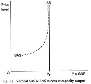
As a result, the short-run aggregate supply curve for the economy as a whole is perfectly horizontal until maximum capacity (full employment) is attained. Once capacity is reached, firms raise their prices to ration the capacity output to those willing to pay the maximum prices. Thus, the economy’s short-run AS curve (SAS) is vertical at full employ­ment.

Fig. 13 illustrates the shape of a Keynesian SAS curve. SAS is completely flat at the existing price level until potential output (Y_F) is reached. In this range, output depends en­tirely on aggregate de­mand. Any change in aggregate demand will lead to a corresponding change in output.

In macroeco­nomics, this horizontal seg­ment is known as the Keynesian range of aggregate supply curve. Once potential capacity is attained, it is not possible to produce more output. So, both SAS and LAS are vertical at the capacity rate of output (Y_F).

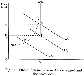
Fig. 14 illustrates the impact of a change in aggregate demand within the rigid assumptions of the Keynesian model. When aggregate demand is less than AD₂ (for example, AD₁), the economy will settle below the full employment.

Since prices and wages are inflex­ible downward, below-capac­ity output rates (Y₁ for example) and abnormally high unemployment will per­sist unless there is an increase in aggregate demand. When output is below its potential, any increase in aggregate de­mand (for example, the shift from AD₁ to AD₂) brings previously idle resources into the productive process at an un­changed price level. In this range, the Keynesian analysis totally disproves Say’s Law. In the Keynesian range, an increase in demand creates its own supply.

Of course, once the economy’s potential output constraint (Y_F) is reached, additional demand would merely lead to higher prices rather than to more output. Since both the SAS and LAS curves are vertical at capacity output, an increase in aggregate demand to AD₃ fails to expand real output further.

The horizontal segment of SAS curve in Fig.14 simply implies that changes in aggregate demand exert little, if any, impact on prices and substantial impact on output when an economy is operating well below capacity. Therefore, under conditions like those of the 1930s — when idle factories and widespread unemployment are present — an increase in aggregate demand will exert its primary impact on output.

On the other hand, the vertical segment of the aggregate supply curve implies that there is an attainable output rate beyond which increases in demand will lead almost exclusively to price increase (and only small increase in real output). So, when aggregate demand is already quite strong (for example, AD₃), increases in aggregate demand will predictably exert their primary impact on prices rather than output.