Difference between Monopoly and Perfect Competition

This article will help you to learn about the difference between Monopoly and Perfect Competition.

Difference between Monopoly and Perfect Competition

(1) In perfectly competitive market, the number of buyers and sellers is very large. There is perfect competition among them. Price is determined for the entire industry by the forces of demand and supply. All firms have to sell their product at that price, No firm can influence price by its single action. It has to accept the price fixed by the industry and to adjust its output to that price.

Thus every firm is a price-taker and quantity- adjuster. There is only one price for a single product in the market at a point of time. On the other hand, the distinction between firm and industry disappears under monopoly because only one firm sells a particular commodity or service. The firm is an industry under monopoly which itself fixes the price for it product. It is, therefore, called a price-maker.

(2) The demand curve or the average revenue curve (AR) of a perfectly competitive firm is a horizontal straight line parallel to the X-axis. In other words, the AR curve of the firm is perfectly elastic and the MR curve coincides with it. But as against this, the AR curve of the monopoly firm slopes downward from left to right and the MR curve is below this.

(3) Despite the similarity between the equilibrium conditions of perfectly competitive firm and monopoly firm, there are dissimilarities between the price- marginal cost relationships. When the under perfectly competitive equilibrium.

MC equals MR, price also equals them at that point because marginal revenue and average revenue coincide with each other and are a straight line curve parallel to the X-axis. In other words, when under perfect competition MC= MR and price also equals them since price (AR) = MR.

Since the AR curve slopes downward to the left under monopoly, the MR curve is below it. So when equilibrium takes place at the point of equality between marginal cost and marginal revenue, price (average revenue) is above the marginal cost, i.e.,

MC = MR < Price (AR)

(4) Another important difference between perfect competition and monopoly is that while under perfect competition the MC curve of the firm must be rising at the point of equilibrium, but it may be rising, falling or constant under monopoly.

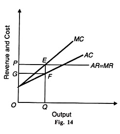
Under perfect competition, it is only possible in the case of left to right upward sloping MC curve since the MR curve is horizontal to the X axis. This equilibrium position is shown in Figure 14 where the firm is in equilibrium at point E. It earns PEFG profits by selling OQ output at OP price.

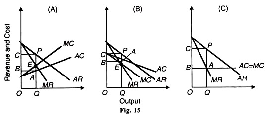
But under monopoly the firm can be in equilibrium with rising, falling or constant MC curve but the MC curve must cut the MR curve from below. This is because the MR curve under monopoly is downward sloping from left to right. The three equilibrium situations are depicted in Figure 15. Panel (A) shows monopoly equilibrium under rising costs where the rising MC curve cuts the MR curve from below at point E.

In Panel (B) a downward sloping MC curve cuts the MR curve from below at point E, while in Panel (C), a horizontal MC (=AC) curve cuts the MR curve from below at point A. In these three situations OP price is determined at which OQ output is sold. But both output OQ and profits РАВС are different in each situation from the other.

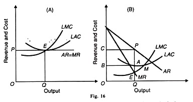
(5) Another difference between perfect competition and monopoly is that in the long-run a competitive form earns only normal profits. The competitive firm can earn more than normal profits in the short-run, see Figure 14. But it is not possible in the long-run because attracted by abnormal profits new firms enter the industry and these profits are competed away, see Figure 16(A).

On the contrary if the monopoly firm is incurring losses in the short-run, it will always earn super-normal profits in the long-run because new firms cannot enter the industry. In Figure 16 (B), the monopoly firm earns PABC super-normal profits.

(6) Another difference between the two market situations relates to their size. In the long-run competitive equilibrium, price equals long-run marginal cost and the minimum long-run average cost, i.e. Price = AR = MR = LMC= LAC at its minimum. This implies that competitive firms in the long-run are of the optimum size and they produce to their full capacity.

While the monopoly firm is of less than the optimum size, because even though the equilibrium point is at the equality of the long-run marginal cost and marginal revenue, yet the long- run average cost curve is not at its minimum point at that level. Both the situations are depicted in Figures 16 (A) and 16 (B).

The competitive equilibrium position is shown in Panel (A) where LMC = MR = AR = LAC at its minimum point E. The firm is of the optimum size. Panel (B) Depicts the equilibrium of the monopoly firm where it is in equilibrium at point E.

But the price ОС (=QP) is not equal to the minimum long-run average cost. The minimum point A/of the LAC curve is to the right of the equilibrium point E. It implies that the monopoly firm possesses excess capacity from E to M and it does not produce to its full capacity.

(7) There is also the difference of price discrimination in the two market situations. The monopolist can charge different prices for the same commodity from his customers, Firstly, because he has no rival, and secondly, when he feels that the elasticity of demand for his product is different in different markets.

But a competitive producer cannot practice price discrimination because the demand curve for his product is perfectly elastic. If he tries to charge a higher price from some of his customers, they will buy the commodity at the market price from some other seller. Thus price discrimination is possible only under monopoly.

(8) Is Monopoly Price higher than Competitive Price? Theoretically, monopoly price is higher than competitive price and the level of output is less than that under competition. The equilibrium of a perfectly competitive industry is determined by the intersection of the industry’s demand (AR) curve and supply (MC) curve.

The supply curve of the competitive industry is the lateral summation of the upward rising portion of the MC curves of the competitive firms in an industry.

A monopolist’s demand curve (AR) also slopes downward to the right. Its corresponding marginal revenue curve (MR) lies below it. Therefore, the equilibrium between the MC curve and the MR curve takes place at a lower level of output. Thus production under monopoly is less than under perfect competition but the monopoly price is higher than competitive price, (AR) > MR = MC.

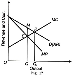
This is depicted in Figure 17 where under perfect competition the equilibrium point P is arrived at by the equality of the demand curve D (AR) and the supply curve MC. At Q₁P price, OQ₁ quantity of the product is bought and sold. On the supposition that the cost conditions are identical both under perfect competition and monopoly, we take these curves for monopoly price determination also.

Accordingly, monopoly equilibrium is at point E the where the MC curve cuts the MR curve, monopoly output is OQ which the monopolist sells at QM price. As is clear from the figure, monopoly price QM is higher than the competitive price Q₁P, but the monopoly output OQ is less than the competitive output OQ₁ If we were to take constant costs, the monopoly output will be exactly half the competitive output. To prove this, we assume identical and constant costs in monopoly firm and competitive industry.

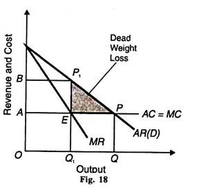
In Figure 18, AR (D) is the demand curve of the competitive industry and AC (=MC) is its supply curve. Both are in equilibrium at point P, so that OQ quantity of the product is bought and sold at the price OP (=OA) under perfect competition.

In this diagram, the mo­nopoly firm is in equilibrium at point E where the MC curve cuts the MR curve from below and the monopoly price Q₁P₁ (= OB) is determined at which output is sold.

As is clear from the diagram, the monopoly price Q₁P₁ is higher than the competitive price QP and the monopoly output OQ₁ is less than the competitive output OQ. The point to be noted is that the monopoly output is exactly half the competitive output. With different demand and cost condition, the monopoly output can be more or less than half the competitive output.

But the monopoly price will be always higher than the competitive price. But it is not essential for the monopoly price to be always higher than the competitive price. It the monopoly firm produces under the law of increasing returns, it enjoys various economies of production and as a result, the cost of production falls. He will, therefore, prefer to sell more at the low price than sell less at a higher price to earn larger profits.

In this situation, the monopoly price can be lower and output larger than under perfect competition.

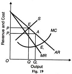
This is illustrated in Figure 19 where AR is the market demand curve for the competitive industry and S is its supply curve. Equilibrium occurs at point E where the two curves intersect each other. OQ quantity is sold at OP price. Now suppose the monopoly firm which was having the same marginal cost curve (S) as that of the perfectly competitive industry, installs a plant which brings in large economies of production.

As a result, its marginal cost curve is everywhere below the 5 curve of the per­fectly competitive industry. This new marginal cost curve is shown as MC which cuts the MR curve from below at the point E₁. At this equilibrium point, the monopoly firm sells more output OQ₁ than the competitive output OQ at a lower price OP₁ than the competi­tive price OP.

(9) The last difference between perfect competition and monopoly is that since the monopoly price is higher than the competitive price, there is loss in consumer’s surplus. This is also explained in terms of Figure 18. Suppose at QP (= OA) price the consumer’s surplus is the area BP₁PA. When the price rises from QP to Q₁P₁ under monopoly, the monopolist takes away BP₁EA area as his profit.

Since the consumer can buy only OQ quantity of the product only at Q₁P₁, price, and he Triangle P_f PE is the net loss in consumer’s surplus. As the consumer is unable to buy Q₁Q quantity of the product (this is not available to him), P₁PE is the net loss in his welfare: BP₁PA – BP₁EA = P₁PE. It is called dead weight loss of the society.