The below mentioned article provides a close view on the measures of dispersion in statistics.
Dispersion Meaning and Classification:
While making any data analysis from the observations given on a variable, we, very often, observe that the degree or extent of variation of the observations individually from their central value (mean, median or mode) is not the same and hence becomes much relevant and important from the statistical point of view.
The necessity is keenly felt in different fields like economic and business analysis and forecasting, while dealing with daily weather conditions, etc. specially in making predictions for future purposes.
The statisticians here prescribe for an well-known concept “dispersion” or the scatteredness or variability of the values of the variable usually from their arithmetic mean. More precisely, it measures the degree of variability in the given observation on a variable from their central value (usually the mean or the median).
ADVERTISEMENTS:
While going in detail into the study of it, we find a number of opinions and definitions given by different renowned personalities like Prof. A. L. Bowley, Prof. L. R. Cannon, Prog. Spiegel, etc. as their own. In this context, we think the definition given by Prof. Yule and Kendall is well accepted, complete and comprehensive in nature as it includes all the important characteristics for an ideal measure of dispersion.
According to them, it should be based on all the given observations, should be readily comprehensible, fairly and easily calculable, be affected as little as possible by sampling fluctuations and amenable to further algebraic treatments.
The following are thus unhesitatingly considered as important characteristics for an ideal measure of dispersion:
(a) It should be rigidly defined,
ADVERTISEMENTS:
(b) It should be easy to calculate and easily understandable,
(c) It should be calculated considering all the available observations,
(d) It should be amenable to further mathematical treatments,
(e) It should be least affected from sampling fluctuations.
The Usual Measures of Dispersion:
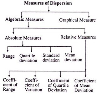
The usual measures of dispersion, very often suggested by the statisticians, are exhibited with the aid of the following chart:
Primarily, we use two separate devices for measuring dispersion of a variable. One is a Algebraic method and the other is Graphical method. In the algebraic method we use different notations and definitions to measure it in a number of ways and in the graphical method we try to measure the variability of the given observations graphically mainly drought scattered diagrams and by fitting different lines through those scattered points.
In the Algebraic method we split them up into two main categories, one is Absolute measure and the other is Relative measure. Under the Absolute measure we again have four separate measures, namely Range, Quartile Deviation, Standard Deviation and the Mean Deviation. And finally, under the Relative measure, we have four other measures termed as Coefficient of Range, Coefficient of Variation, Coefficient of Quartile Deviation and the Coefficient of Mean Deviation.
Absolute Measures of Dispersion:
1. Range: The simplest and the easiest method of measuring dispersion of the values of a variable is the Range. It is measured just as the difference between the highest and the lowest values of a variable. The extent of dispersion increases as the divergence between the highest and the lowest values of the variable increases.
We thus express the magnitude of Range as:
Range = (highest value – lowest value) of the variable.
For determining Range of a variable, it is necessary to arrange the values in an increasing order.
It will enable us to avoid mistakes in calculation and give us the best result.
Let us consider two separate examples below considering both the grouped and the ungrouped data separately.
ADVERTISEMENTS:
Example 1:
Consider the following series of numbers:
1, 2, 4, 6, 8, 10, 12.
Solution:
ADVERTISEMENTS:
Here, the highest value of the series is 12 and the lowest is 1.
Therefore, the Range = 12 – 1 = 11 i.e. the values of the variable are scattered within 11 units.
Example 2:
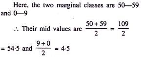
For the data presented with their respective frequencies, the idea is to measure the same as the difference between the mid-values of the two marginal classes.
ADVERTISEMENTS:
Consider the following table:
The required Range is 54.5 – 4.5 = 50 or the observations on the variable are found scattered within 50 units.
It is to be noted that any change in marginal values or the classes of the variable in the series given will change both the absolute and the percentage values of the Range.
At times of necessity, we express the relative value of the Range without computing its absolute value and there we use the formula below
ADVERTISEMENTS:
Relative value of the Range = Highest value – Lowest value/Highest value + Lowest value
In our first example the relative value of the
Range is = 12-1/12+1 = 11/13 = 0.84
The ‘Range’, as a measure of ‘Dispersion’, has a number of advantages and disadvantage. The concept of Range is, no doubt, simple and easy enough to calculate, specially when the observations are arranged in an increasing order. But the main disadvantage is that it is calculated only on the basis of the highest and the lowest values of the variable without giving any importance to the other values.
Therefore, the result can only be influenced with changes in those two values, not by any other value of the variable. Again, in the case of a complex distribution of a variable with respective frequencies, it is not much easy to calculate the value of Range correctly in the above way. For all these reasons.
Range as a measure of the variability of the values of a variable, is not widely accepted and spontaneously prescribed by the Statisticians of today However, it is not totally rejected even today as it has certain traditional accept abilities like representing temperate variations in a day by recording the maximum and the minimum values regularly by the weather department, while imposing controlling measures against wide fluctuations in the market prices of the essential goods and services bought and sold by the common people while imposing Price-control and Rationing measures through Public Sector Regulations, mainly to protect interests of both the buyers and sellers simultaneously.
ADVERTISEMENTS:
2. Quartile Deviation: While measuring the degree of variability of a variable Quartile Deviation is claimed to be another useful device and an improved one in the sense it gives equal importance or weightage to all the observations of the variable. Here the given observations are classified into four equal quartiles with the notations Q1, Q2, Q3 and Q4. The average value of the difference between the third and the first quartiles is termed as the Quartile Deviation.
Symbolically, we write:
Quartile Deviation = Q3 – Q1/2
Through this measure it is ensured that at least 50% of the observations on the variable are used in the calculation process and with this method the absolute value of the Quartile Deviation can easily be measured.
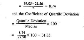
For determining the proportionate Quartile Deviation, also called the Coefficient of Quartile Deviation, we use the following formula:
Coefficient of Quartile Deviation:
Consider the following examples:
Example 1:
Calculate the Quartile Deviation and Co-efficient of Quartile Deviation from the following data:
8, 10, 12, 14, 16, 18, 20.
Solution:
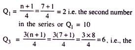
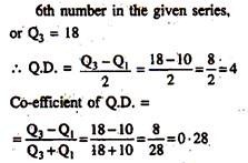
Here, n = 7, the first and third quartiles are:
Example 2:
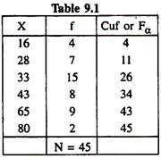
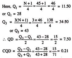
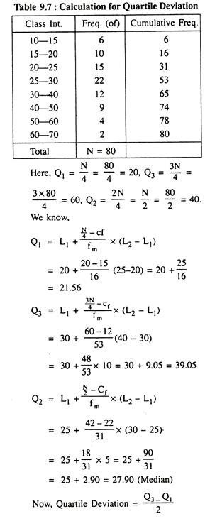
Determine the QD and CQD from the following grouped data:
Solution:
In order to determine the values of QD and Co-efficient of QD Let us prepare the following table:
Grouped frequency distribution of X with corresponding cumulative frequencies (Fα).
Advantages and disadvantages of Quartile Deviation:
Advantages:
(a) Quartile Deviation is easy to calculate numerically.
(b) Calculation for QD involves only the first and the third Quartiles.
(c) It can be used safely as a suitable measure of dispersion at all situations.
(d) It remains unaffected from the extreme values of the variable.
(e) It can be calculated readily from frequency distributions with the open end classes.
(f) QD at least is a better measure of dispersion compared to Range.
Disadvantages:
(a) Quartile deviation as a measure of dispersion is not much popularly prescribed by the statisticians.
(b) It is used only in rare cases.
(c) It is not a reliable measure of dispersion as it ignores almost (50%) of the data.
3. Standard Deviation: The concept of SD as a successful measure of dispersion was introduced by the renowned statistician Karl Pearson in the year 1893 and it is still recognised as the most important absolute measure of dispersion.
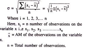
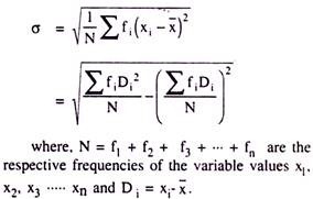
SD of a set of observations on a variable is defined as the square root of the arithmetic mean of the squares of deviations from their arithmetic mean. In other words it is termed as “The Root- Mean-Squared-Deviations from the AM” Again, it is often denoted as the positive square root of the variance of a group of observations on a variable.
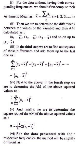
It is usually expressed by the Greek small letter ‘σ’ (pronounced as Sigma) and measured for the information without having frequencies as:
But, for the data having their respective frequencies, it should be measured as:
The following six successive steps are to be followed while computing SD from a group of information given on a variable:
Like the other measures of dispersion SD also has a number of advantages and disadvantages of its own.
Let us enlist them in order below:
Advantages:
(a) Calculation of SD involves all the values of the given variable.
(b) It uses AM of the given data as an important component which is simply computable.
(c) It is least affected by sampling fluctuations.
(d) It is easily usable and capable of further Mathematical treatments.
(e) It is well defined.
(f) It is taken as the most reliable and dependable device for measuring dispersion or the variability of the given values of a variable.
(g) Statisticians very often prescribe SD as the true measure of dispersion of a series of information.
(h) It can tactfully avoid the complication of considering negative algebraic sign while calculating deviations.
Disadvantages:
(a) It involves complicated and laborious numerical calculations specially when the information are large enough.
(b) The concept of SD is neither easy to take up, nor much simple to calculate.
(c) It is considerably affected by the extreme values of the given variable.
(d) To compute SD correctly, the method claims much moments, money and manpower.
Therefore, the SD possesses almost all the prerequisites of a good measure of dispersion and hence it has become the most familiar, important and widely used device for measuring dispersion for a set of values on a given variable.
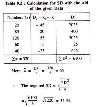
Example 1:
Calculate SD of the following numbers:
20, 85, 120, 60 and 401
Solution:
We can represent AM of the given number as:
Now, we calculate the desired SD through the following exercise:
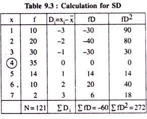
Example 2:
Find the SD for the following distribution:
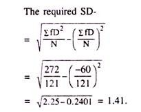
Solution:
To calculate SD of the given distribution, we reconstruct the following table:
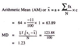
4. Mean Deviation: Practically speaking, the Range and the Quartile deviation separately cannot provide us the actual measurement of the variability of the values of a variable from their mean because they cannot ideally express the central value and the extent of scatteredness of those values around their average value. Moreover, these measures are not prepared on the basis of all the observations given for the variable. In order to avoid such limitations, we use another better method (as it is claimed) of dispersion known as the ‘Mean Deviation’.
Conventionally, it is denoted by another Greek small letter Delta (∆), also known as the ‘average deviation.’
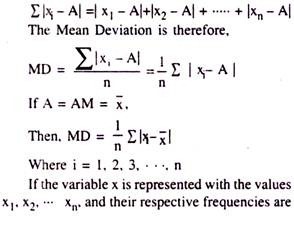
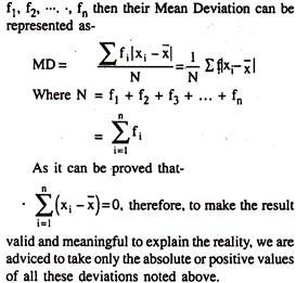
By definition it is the Arithmetic mean of the absolute deviations of the individual values of the given variable from their average value (normally the mean or the median). It is thus considered as an Absolute Measure of Dispersion.
Method of Computation:
Consider x to be a variable having n number of observations x1, x2, x3, ……. xn and A to be its arithmetic mean or the middle most value i.e., the median, then the absolute (or positive) values of the deviations of all these observations from A and their sum can be represented as:
Advantages of the MD:
(a) On many occasions it gives fairly good results to represent the degree of variability or the extent of dispersion of the given values of a variable as it takes separately all the observations given into account.
(b) It can also be calculated about the median value of those observations as their central value and then it gives us the minimum value for the MD
(c) In usual situations, it is calculated taking deviations from the easily computable arithmetic mean of the given observations on the variable.
(d) It is easy to calculate numerically and simple to understand.
Disadvantages of the MD:
(a) The main complaint against this measure is that it ignores the algebraic signs of the deviations.
(b) It is not generally computed taking deviations from the mode value and thereby disregards it as another important average value of the variable.
(c) It is rarely used in practical purposes.
Example 1:
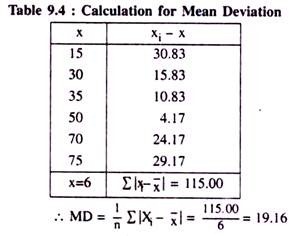
(i) Calculate mean deviation about Arithmetic Mean of the following numbers:
35, 70, 15, 75, 30, 50
Solution:
Let us arrange the numbers in an increasing order as 15, 30, 35, 50, 70, 75 and compute their AM as:
AM = 15 + 30 + 35 + 50 + 70 + 75/6 = 275/6
= 45.83.
Now, we convert the data into:
Example 2:
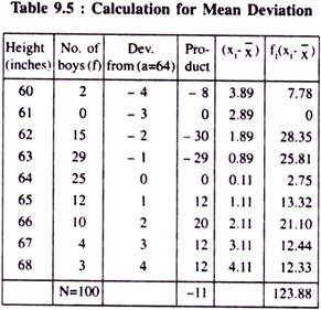
Calculate the Mean Deviation for the following data:
Solution:
To calculate MD of the given distribution, we construct the following table:
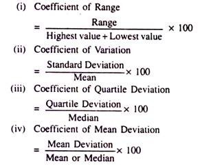
Relative measures of Dispersion:
While studying the variability of the observations of a variable, we usually use the absolute measures of dispersion namely the Range, Quartile deviation. Mean deviation and Standard deviation. But, the results of such measures are obtained in terms of the units in which the observations are available and hence they are not comparable with each other. Moreover, the results of the absolute measure gets affected by the number of observations obtainable on the given variable as they consider only the positive differences from their central value (Mean/Median).
To eliminate all these deficiencies in the measurement of variability of the observations on a variable, we accept and introduce in respective situations the very concept of the Relative measures of dispersion as they are independent of their own units of measurement and hence they are comparable and again can be examined under a common scale when they are expressed in unitary terms. Here lies the superiority of the Relative Measures over the Absolute Measures of dispersion.
The usual Relative Measures of Dispersion are:
Among these four coefficients stated above the Coefficient of Variation is widely accepted and used in almost all practical situations mainly because of its accuracy and hence its approximation to explain the reality.
Example 1:
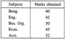
Determine the Coefficient of Range for the marks obtained by a student in various subjects given below:
Solution:
Here, the highest and the lowest marks are 52 and 40 respectively.
Hence, Range = 52 – 40 = 12.
The Coeff. of Range = 12/52+40×100
Example 2:
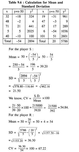
The performances of two Batsmen S and R in five successive one-day cricket matches are given below.
Identify the batsman who is more consistent:
Solution:
Here, we can use ‘Coefficient of Variation’ as the best measure of dispersion to identify the more consistent one having lesser variation. As the components of CV, we are to derive first the Mean and the Standard Deviation of the scores obtained by the two Batsmen separately using the following usual notations:
Let us prepare the following table for finding out Mean and SD of the given information:
For the cricketer S the Coefficient of Variation is smaller and hence he is more consistent.
Example 3:
Calculate the Coefficient of Quartile Deviation from the following data:
Solution:
To calculate the required CQD from the given data, let us proceed in the following way:
Example 4:
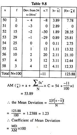
Compute the Coefficient of Mean-Deviation for the following data:
To calculate the coefficient of MD we take up the following technique.
Solution:
Calculation for the Coefficient of Mean-Deviation.
A Comparative Analysis among the Usual Measures of Dispersion:
Statisticians together unanimously opines that an ideal measure of dispersion should possess certain necessary characteristics.
Let us now enlist them below:
(a) The principle followed and the formula used for measuring the result should easily be understandable.
(b) The numerical value of the required dispersion should easily be computable.
(c) The definition and the concept of dispersion should be complete and comprehensive enough.
(d) The algebraic treatment used in the process should easily be applicable elsewhere.
(e) The relevant measure of dispersion should try to include all the values of the given variable.
(f) The result finally achieved should be least affected by sampling fluctuations.
On the basis of the above characteristics we now can examine chronologically the usual measures of dispersion and identify the best one in the following way:
In the light of the above criteria when we examine Range as a measure of dispersion, we find that it is no doubt easy to calculate but does not include all the values of the given variable and further algebraic treatments cannot be applied with it in other Statistical analyses. Again, the concept of Range cannot provide us any idea about the nature of distribution of the concerned variable and practically it is not possible for us to determine the final result for opened classes. For these limitations, the method is not widely accepted and applied in all cases.
Compared to Range, Quartile Deviation, no doubt, is a better measure of dispersion and it is also easy to calculate. While computing the result it involves larger information than the Range. The result will not be affected even when the distribution has an open end. Again, it has least possibility to be affected remarkable by an individual high value of the given variable. However, the method neither include all the values of the variable given in the exercise, nor it is suitable for further algebraic treatments. For all these reasons the method has its limited uses.
The Mean Deviation, for its own qualities, is considered as an improved measure of dispersion over Range and Quartile deviation as it is able to provide us a clear understanding on the very concept of dispersion for the given values of a variable quite easily. It is not only easy to compute, it takes into account all the given values of the variable and again the final result remains almost unaffected from any remarkably high value of the variable under consideration.
When we use the Arithmetic mean instead of the Median in the process of calculation, we get a rough idea on the nature of distribution of the series of observations given for the concerned variable. But the greatest objection against this measure is that it considers only the absolute values of the differences in between the individual observations and their Mean or Median and thereby further algebraic treatment with it becomes impossible.
Again, the use of Median while measuring dispersion of the values of a variable produces incorrect result on many occasions because computation of the Median value from the given observations usually include considerable errors when the observations represent wide disparity among themselves.
The Standard Deviation, as a complete and comprehensive measure of dispersion, is well accepted by the statisticians specially because it possesses simultaneously all the qualities unhesitatingly which are required for an ideal measure of dispersion. Its definition is complete and comprehensive in nature and it involves all the given observations of the variable.
Further algebraic treatments can also be applied easily with the result obtained afterwards. If we are provided with homogeneous or equivalent observations on two or more but not on unlimited number of variables with their own standard deviations, we can easily derive their combined standard deviation.
Lorenz Curve – The curve of concentration:
To study the exact nature of a distribution of a variable provided with a number of observations on it and to specify its degree of concentration (if any), the ‘Lorenz Curve’ is a powerful statistical device. This type of a curve is often used as a graphical method of measuring divergence from the average value due to inequitable concentration of data. It is thus known as the ‘Curve of Concentration’. Statistically speaking, it is a cumulative percentage curve which shows the percentage of items against the corresponding percentage of the different factors distributed among the items.
With a view to tracing out such a curve, the given observations are first arranged in a systematic tabular form with their respective frequencies and the dependent and independent variable values are cumulated chronologically and finally transformed into percentages in successive columns and plotted on a two dimensional squared graph paper. The locus of those points ultimately traces out the desired ‘Lorenz Curve’,
Economists and other social scientists very often opine that inequality in the distribution of income and wealth among the individuals in a society is a common phenomenon today all over the world mainly due to our aimless and unbalanced growth policies framed by the concerned authorities, called ‘growth without development’ today in economics, resulting in rise in GDP but no significant rise in the per-capita income of the people at large.
To study the extent or the degree of economic inequality prevailing among the people of various professional categories, construction of a ‘Lorenz Curve’ and estimation of the ‘Gini Co-efficient’ is the order of the day as it helps the planners to take effective future development policies for the people indiscriminately. Let us offer a suitable example of it to measure such a degree of income inequality persisting among the weavers of Nadia, W.B. from a research paper relevant in this context.
Measurement of Economic Inequality among the Weavers of Nadia, W.B:
Here, we are interested to study the nature and the exact degree of economic inequality persisting among these workforces. This is usually displayed in terms of inequalities existing in the distribution of income and wealth among the people under consideration. Let us analyse this phenomenon in terms of a study based on the distribution of personal incomes of the chosen sample respondents that is how the total income of the entire workforce is shared by the different income classes.
The well-known statistical device to exhibit this kind of a ground level reality is to trace out a ‘Lorenz-Curve’, also called the Curve of Concentration and measure the exact nature and degree of economic inequality existing among the weavers of Nadia with the aid of ‘GINI- COEFFICIENT’, an unit free positive fraction (lying in between 0 and 1).
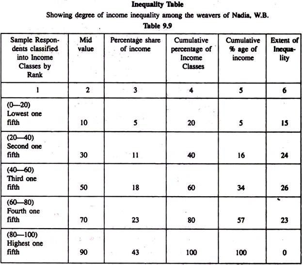
Let us represent our numerical findings in this context from the available data in the following tabular form:
(An exclusive survey over 222 weavers at random in 5 important weaving centres which is 15% of the total number of weavers engaged in those areas as prescribed in the Sampling Theory.)
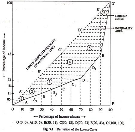
The table represented above shows that the poorest 20 per cent of the income earners receive only 5 per cent of the total income whereas the richest 20 per cent of the sample respondents shared as much as 43 per cent of it. This undoubtedly depicts a clear picture of high degree of income- inequality prevailing among our sample respondents. Again, the second lowest 20 per cent weavers have got a mere 11 per cent the third 20 per cent shared only 18 per cent and the fourth 20 per cent about 23 per cent of the total income.
In March-April, 2001-02, with the aid of the above figures, we can now derive the required ‘Lorenz-Curve’ in the following way: Here, the Gini Coefficient (G)
The result finally obtained (G=0.60) thus implies the fact that a high degree of economic inequality is existing among the weavers of Nadia, W.B.
Here, we have plotted these information on a two dimensional plane showing percentage of income-classes horizontally and the corresponding percentage of income received vertically. The locus that we have traced out here as O-A-B-C-D-E-0 is called the ‘LORENZ-CURVE’. This curve actually shows the prevailing nature of income distribution among our sample respondents.
The dotted area depicted above this curve indicates the exact measure of deviation from the line of ‘Absolute-Equality’ (OD’) or the ‘Egalitarian-Line’ (dotted Line) and hence gives us the required measure of the degree of economic inequality persisting among the weavers of Nadia, W.B. that becomes evident from the above income distribution.
