4 Types of Duopoly Models (With Diagram)

The uncertainty is respect of behaviour pattern of a firm under oligopoly arising our of their unpredictable action and reaction makes a systematic analysis of oligopoly difficult.

However, classical and modern economists have developed a variety of models based on different behavior assumptions.

These models can broadly be classified into two categories (I) classical duopoly models and modern oligopoly Duopoly Models, when there are only two sellers a product, there, exists duopoly.

Duopoly is a special case of oligopoly. Duopoly is a special case in the sense that it is limiting case of oligopoly as there must be at least two sellers to make the market oligopolistic in nature.

1. The Cournot’s Duopoly Model

2. The Chamberlin Duopoly Model

3. The Bertrand’s Duopoly Model

4. The Edgeworth Duopoly Model

1. Cournot’s Duopoly Model:

Augustin Cournot, a French economist, was the first to develop a formal duopoly model in 1838.

To illustrate his model, Cournot assumed:

(a) Tow firms, each owing an artesian mineral water well;

(b) Both operate their wells at zero marginal cost²;

(c) Both face a demand curve with constant negative slope;

(d) Each seller acts on the assumption that his competitor will not react to his decision to change his and price. This is Cournot’s behavioural assumption.

On the basis of this model, Cournot has concluded that each seller ultimately supplies one-third of the market and charges the same price. While one-third of the market remains unsupplied.

Diagram Representation:

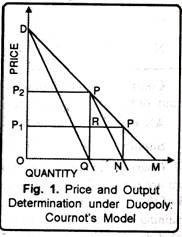
Cournot’s duopoly model is presented in Fig. 1. To begin the analysis, suppose that there are only two firms. A and B, and that, initially. A is the only seller of mineral water in the market. In order to maximize his profits (or revenue), he sells quantity OQ where his MC = O MR, at price OP₂ His total profit is OP₂PQ.

Now let B enters the market. The market open to him is QM which is half of the total market. He can sell his product in the remaining half of the market. He assumes that A will not change his price and output as he is making the maximum profit i.e., A will continue to sell OQ at price OP₂ Thus, the market available to B is QM and the demand curve is PM.

When to get maximize revenue, B sells ON at price OP1, His total revenue is maximum at QRP’N. Note that B supplies only QN = 1/4 = (l/2)/2 of the market.) With the entry of B, price falls to OP₁ Therefore, A’s expected profit falls to OP₁ PQ Faced with this situation, A attempts to adjust his price and output to the changed conditions. He assumes that B will not change his output QN and price OP₁ as he is making maximum profit.

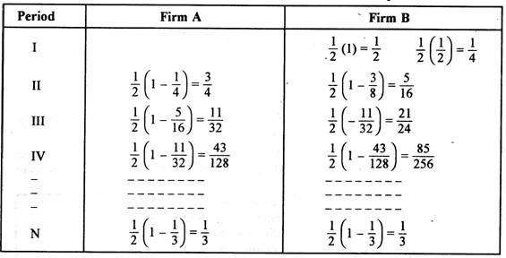
Accordingly, A assumes that B will continue to supply 1/4 of market and he has 3/4 (= 1 – 14) of the market available to him. To maximise his profit. Supplies 1/2 of (3/4), i.e., 3/8 of the market. Note that A’s market share has fallen from 1/2 to 3/8.

Now it is B’s turn to react. Considering Cournot’s assumption, B assumes that A will continue to supply only 3/8 of the market and market open to him equals 1 – 3/8 = 5/8.

In order to maximise his profit under the new conditions B supplies 1/2 x 5/8 = 5/16 of the market. It is now for A to reappraise the situation and adjust his price and output accordingly.

This process of action and reaction continues in successive periods. In the process, A continues to lose his market share and B continues to gain. Finally situation is reached when their market shares equal at 1/3 each.

Any further attempt to adjust output produces the same result. The firms, therefore, reach their equilibrium position where each one supplies one-third of the market.

The equilibrium of firms, according to Cournot’s model, has been presented in table below:

Cournot’s equilibrium solution is stable. For given the action and reaction, it is not possible for any of the two sellers to increase their market share.

It can be shown as follows:

A’s share= 1/2(1 – 1/3) = 1/3.

Similarly B’s share = 1/2 (1 – 1/3) = 1/3.

Cournot’s model of duopoly can be extended to the general oligopoly. For example, if there are three sellers, the industry, and firms will be in equilibrium when each firm supplies 1/3 of the market. Thus, the three sellers together supply 3/4 of the market, 1/4 of the market remaining unsupplied. The formula for determining the share of each seller in an oligopolistic market is: Q -f- (n + 1), where Q = market size, and n = number of sellers.

Criticism of the Model:

Although ournot’s model yields a stable equilibrium, it has been criticised on the following grounds:

(1) Curnot’s behavioural assumption [assumption (d) above] is naive to the extent that it implies that firms continue to make wrong calculations about the competitor’s behaviour. Each seller continues to assume that his rival will not change his output even though he reportedly observes that his revel firm does change its output.

(2) The assumption of zero cost of production is totally unrealistic. If this assumption is dropped, it does not alter his position.

2. Chamberlin’s Duopoly Model- A Small Group Model:

Chamberlin’s model of duopoly recognizes interdependence if firms in such a market. Chamberlin argues that in the real world of oligopoly firms are not so native that they will not learn from the past experience. However, he makes the same assumptions as the exponents of old classical models have done. In other words, his model is also based on the assumption of homogeneous products, firms of equal size with identical costs, no entry by new firms and full knowledge of demand.

Recognition of interdependence of firms in an oligopolistic market given us a result quite different from that of Cournot. Chambrilin argues that firms are aware of the fact that their output or price decision will definitely invite reactions of other firms. Therefore, he goes not visualize any price war in oligopolistic markets. He also rules out the possibility of firms adjusting their outputs over a period of time and thus reaching the equilibrium at an output level lower than that would be reached under monopoly.

According to Chamberlin, recognition of possible sharp reactions to an oligopolistic firm’s price or output manipulations would avert harmful competition amongst the firms in such a market and would result in a stable industry equilibrium with the monopoly price and monopoly output. He further stated that no collusion is required for obtained this solution.

In case farms in an oligopolistic market are aware of their mutual dependence, and willing to learn from their past experience, then in order to maximize their individual and joint profits they will charge the monopoly price.

Chamberlin’s model can be explained in the frame work of a dupoly market. Chamberlin, like Cournot, assumes linear demand for the product. For simplicity we assume that even in this case the cost of producing the good is zero.

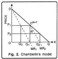
Chamberlin model has been illustrated in Figure 2. In this figure DQ is the market demand curve. If firm A is first to enter the market, it will produce output OQ₁ because at this level of output its marginal revenue is equal to marginal cost (MR = MC = 0). The firm can charge price OP₁ which is the monopoly price.

This will maximise its profits. At price OP) elasticity of demand is unity. Firm B entering market at this stage considers that its demand curve is CQ and will thus produce Q₁Q₂ so as to maximise its profit. It will charge price OP₂.

It now realizes that it cannot sell QQ₁ quantity at the monopoly price and thus decides to reduce the output to QQ₃, which is one-half of the monopoly output QQ₁. Firm B can continue to produce quantity Q₁Q₂ which is same as Q₃Q₁.

The industry output thus is OQ₁ and the price rises to the level OP₁. This is an ideal situation from the point of view of both firms A and B. In this case, the joint output of the two firms is monopoly output and they charge monopoly price. Thus, considering the assumption of equal costs (costs = 0) the market will be shared equally between firms A and B.

Appraisal of the Model:

Chamberlin’s model is certainly more realistic than earlier models. It assumes that firms recognize interdependence and then act in a manner that monopoly solution is reached. In the real world of oligopoly there are certain difficulties in reaching this solution. In the absence of collusion, firms must have a good knowledge of market demand curve which is almost impossible to obtain. In case this information is lacking, firms will not know how to reach monopoly solution.

Further, Chamberlin ignores entry. In real practice, oligoplistic markets are rarely closed. So if we recognize the fact of entry, it would not be certain that the stable monopoly solution will ever be reached. Differences in costs and market opportunities are also hindrance for attaining a monopoly-type outcome by the independent actions of firms in oligopolies.

3. Bertrand’s Duopoly Model:

Bertrand, a French Mathematician developed his own model of duopoly in 1883. Bertrand’s model differs from Cournot’s model in respect of its behavioural assumption. While under Cournot’s model, each seller assumes his rival’s output to remain constant, under Bertrand’s model each seller determines his price on the assumption that his rival’s price, rather than his output, remains constant.

Bertrand’s model focuses on price competition. His analytical tools are reaction function of the duopolists. Reaction functions are derived on the basis of iso-profit curves. An iso-profit curve, for a give level of profit, is drawn on the basis of various combinations of prices charged by the rival firms. He assumed only two firms, A and B and their prices are measured along the horizontal and vertical axes, respectively.

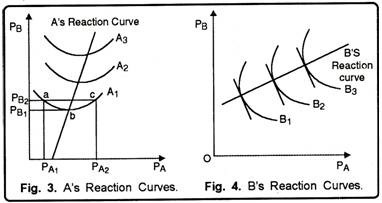
Their iso-profit curves are drawn on the basis of the prices of the two firms. Iso-profit curves of the two firms are concave to their respective prices axis, as shown in Fig. 3 and 4. Iso- profit curves of firm A are convex to its price axis P_A (Fig. 3) and those of firm B are convex to P_B (Fig. 4).

In Figure 4, we have curve A, which shows that A can earn a given profit from the various combinations of its own and its rival’s price. For example, price combinations at points, a, b and c yield the same level of profit indicated by the iso-profit curve A₁. If firms B fixes its prices Pb₁– firm A has two alternative prices, Pa₁ and Pa₂, to make the same level of profits.

When B reduces its price, A may either raise its price or reduce it. A will reduce its price when he is at point c and raise its price when he is at point a. But there is a limit to which this price adjustment is possible. This point is shown by point b. So there is a unique price for A to maximize its profits. This unique price lies at the lowest point of iso-profit curve.

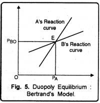
The same analysis applies to all other iso-profit curves, A₁ A₂ and A3 we get A’s reaction curve. Note that A’s reaction curve has a rightward slant. This is so because, iso-profit curve tends to shift rightward when A gains market from his rival B.

Following the same process, B’s reaction curve may be drawn as shown in Fig. 4.

The equilibrium of duopolists suggested by Bertrand’s model may be obtained by putting together the reaction curves of the firms A and B as shown in Fig. 5.

The reaction curves of A and B intersect at point E where their expectations materialize, point E is therefore equilibrium point. This equilibrium is stable. Fo, if any one of the firms disagrees to this point, it will create a series of actions and reactions between the firms which will lead them back to point E.

Criticism of the Model:

Bertrand’s model has been criticised on the same grounds as Cournot’s model. Bert- rand’s implicit behavioural assumption that firms never learn from their past experience seems to be unrealistic. If cost is assumed to be zero, price will fluctuate between zero and the upper limit of the price, instead of stabilizing at a point.

4. Edgeworth’s Duopoly Model:

Edgeworth developed his model of duopoly in 1897. Edgeworth’s model follows Bertrand’s assumption that each seller assumes his rival’s price, instead of his output, to remain constant.

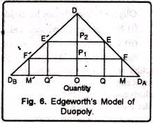
His model is illustrated in Fig. 6.

In this figure we have supposed that there are two sellers, A and B, in the market who face identical demand curves. A has his demand curve DD_B and as DD_B Let us also assume that seller A has a maximum capacity of output OM and B has a maximum output capacity of OM’. The ordinate ODA measures the price.

To explain Edgeworth’s model, let us assume, to begin with, that A is the only seller in the market. Following the profit maximising rule of a monopoly seller, he sells OQ and charges a price, OP₂. His monopoly profit under zero cost, equals OP₂EQ Now, let B enter the market. B assumes that A will not change his price since he is making maximum profit. He sets his price slightly below A’s price (OP₂) and is able to sell his total output. At this price, he captures a substantial part of A’s market.

Seller A, on the other hand, that his sales have gone down. In order to regain his market, A sets his price slightly below B’s price. This leads to price-war between the sellers.

The price- war takes the form of price-cutting which continues until price reaches OP₁ At this price both A and B are able to sell their entire output- A sells OQ and B sells OQ The price OP₁ could therefore be expected to be stable. But, according to Edgeworth, price OP₁ should not be stable.

Simple reason is that, once price OP is set in the market, the sellers observe an interesting fact. This is, each seller realise that his rival is selling his entire output and he will therefore not change his price, and each seller thinks that he can raise his price to OP₂ and can make pure profit.

This realisation forms the basis of their action and reaction. For examples, let seller A take the initiative and raise his price to OP₂. Assuming A to retain his price OP₂.B finds that if he raises his price at a level slightly below OP₂ he can sell his entire output at a higher price and make greater profit. Therefore, B raises his price according to his plan.

Now it is A’s turn to know the situation and react. A finds that his price is higher than B’s price and his total sale has fallen. Therefore assuming B to retain his price, A reduces his price slightly below B’s price.

Thus, the price-war between A and B begins once again. This process continues indefinitely and price keeps moving up and down between OP₁ and OP₂ Obviously, according to Edgeworth’s model of duopoly, equilibrium is unstable and indeterminate since price and output are never determined. In the words form Edgeworth, “there will be an indeterminate tract through which the index of value will oscillate, or, rather will vibrate irregularly for an indefinite length of time.

In a net shell Edgeworth’s model, like Cournot’s is based on a native assumption, i.e. each seller continues to assume that his rival will never change his price even though they are proved repeatedly wrong. But according to Hotelling Edgeworth’s model is definitely an improvement upon Cournot’s model in that it assumes price, rather than output, to be the relevant decision variable for the sellers.