Top 3 Models of Duopoly (With Diagram)

The following points highlight the top three models of duopoly. The models are: 1. The Cournot Model 2. The Stackelberg Model 3. The Chamberlin Model.

Duopoly Model # 1. The Cournot Model:

The oldest determinate solution to the duopoly problem is by the French economist, A.A. Cournot in 1838, who took the case of two mineral water springs situated side by side and owned by two firms A and B.

Assumptions:

The Cournot model is based on the following assumptions:

(1) There are two independent sellers. In other words, interdependence of the duopolists is ignored.

(2) They produce and sell a homogeneous product, mineral water.

(3) The total output must be sold out, being perishable and non-storable.

(4) The number of buyers is large.

(5) Each seller knows the market demand curve for the product.

(6) The cost of production is assumed to be zero.

(7) Both have identical costs and identical demands.

(8) Each seller decides about the quantity he wants to produce and sell in each period.

(9) But each is ignorant about his rival’s plan about output.

(10) At the same time, each seller takes the supply or output of its rival as constant.

(11) Neither of them fixes the price for its product, but each accepts the market demand price at which the product can be sold.

(12) The entry of firms is blocked.

(13) Each seller aims at obtaining the maximum net revenue or profit.

Explanation:

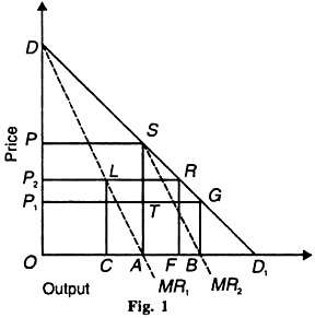
Given these assumptions, suppose there are two mineral water springs exploited by two firms, A and B. The market demand curve is DD₁, and its marginal revenue curve is MR, as shown in Figure 1. The marginal costs of both A and В are assumed to be zero so that they coincide with the horizontal axis.

Suppose firm A is the only producer in which case it produces and sells OA (=½ OD₁) quantity when it’s MR, equals its marginal cost curve (horizontal axis) at point A. It charges the monopoly price AS (=OP) and earns ОASP as monopoly profits.

Now firm В enters the market and expects that A will not change its output level OA. It, therefore, regards SD₁ segment of the market demand curve as its demand curve. Its corresponding marginal revenue curve is MR₂ which intersects the horizontal axis (its marginal cost curve) at point B. Thus it produces and sells AB (= ½ AD₁ = BD₁) quantity at BG (=OP₁) price and it expects to earn BGTA profits.

Firm A finds that with the entry of B, price has fallen to OP₁ from OP. As a result, its expected profits decline to OP JA. In this situation, it tries to adjust its price and output. Accordingly, assuming that В will continue to sell the same quantity AB (=BD₁), it regards the remaining portion of the market OB available to it. It thus sells ½OB. The reduction in its output from OA (=½OD₁) to AB (= ½ OB) causes the price to rise (not shown in the figure to simplify the analysis).

As a result of A’s reduction in output, В thinking that A will continue to produce less, reacts by increasing its output to ½(OD₁-AB) which causes the price to fall. In this way, A’s reducing its output and causing the price to rise, and B’s reaction in increasing its output and causing the price to fall, will ultimately lead to an equilibrium price OP₂. At this price, the total output of mineral water is OF, which is equally divided between the two firms.

Each duopolist sells 1/3 of the market i.e. A sells ОС and В sells CF. At this price, A’s OCLP₂ equal that of B’s profits CFRL. It is evident that both the producers sell 2/3 of the total output, OD₁ and each is producing 1/3 of OD₁.

Let us compare the Cournot duopoly solution with the perfectly competitive solution. The duopoly firms A and В in equilibrium charge OP₂ price and sell OF output. Under perfect competition, the total output will be OD at zero prices. The price is zero because the marginal cost is zero. When the MR₁ curve intersects the horizontal axis, which is the MC curve, the price is zero at point A in the figure.

The total output OD₁ will be divided between A and В equally as OA and AD₁ Notice that in the Cournot solution, the price OP₂ exceeds the zero marginal cost and zero prices under perfect competition, and the output OF is less than OD₁ under perfect competition. However, in the Cournot solution the output (OF) is greater than it would be under monopoly (OA). But the price under monopoly (OP) would be higher than under the Cournot solution (OP₂).

Conclusion:

The Cournot model can be extended even to more than two firms. As more and more firms enter the oligopoly industry, the equilibrium output and price of the industry will approach the perfectly competitive output OD₁ and the zero prices.

Its Criticisms:

The cournot model has been criticised on the following grounds:

1. The main defect in Cournot’s solution is that each seller assumes his rival’s supply fixed, despite repeatedly observing changes in it. Joseph Bertrand, a French mathematician, criticising Cournot in 1883 pointed out that seller A in order to regain all the customers lost to B, will fix a price slightly below that fixed by В and price cutting may continue until the price becomes zero. Thus, Bertrand argued that there would not be any limit to the fall in price since each seller could by doubling his produce, and underbid his rival. This would tend to drive down the price to the competitive level in the long-run.

2. The model is silent about the period within which one firm reacts and adjusts its output to the moves of the other. Thus it is a static model.

3. The Cournot solution is unrealistic because it assumes zero cost of production.

4. It is a closed model because it does not allow entry of firms.

5. The assumption that each duopolist can act without any output reaction from the other is unrealistic. It is, in fact, a no-learning-by-doing model.

6. Marshall, therefore, regarded Cournot’s model as “incapable of a universal solution.” This is because it is not possible to find an actual duopoly market where each duopolist acts autonomously and output is the ‘sole parameter of action’.

Duopoly Model # 2. The Stackelberg Model:

The German economist Stackelberg proposed a solution to the duopoly problem based on the assumption that each seller recognises the interdependence of other’s actions. Each seller either regards himself a leader or a follower. Each seller determines the maximum profits he can get both by being a leader and a follower.

He will then choose to play whatever role brings him greater profits. Thus there is market equilibrium if their desires are consistent to each other. The Stackelberg solution is based on the reaction curves. Each reaction curve expresses the output of each seller as a function of his rival’s output.

Thus if Q_A is the output of seller A and Q_B of seller B, then the reaction function of seller A is Q = f (Q_B) and that of В is Q_B = F (Q_A). These reaction functions are derived from the profit indifference maps of the individual duopolists. Thus A’s reaction function gives the value of Q_A which maximises A’s profit for any specified value of B’s output (Q_B).

Similarly, for any specified value of A’s output, the corresponding value of B’s output maximises B’s profit. This is illustrated in the following figures where the leadership point L_A of seller A is shown to lie on the reaction curve of firm B, and the leadership point L_B of seller В is shown to lie on the reaction curve of firm A. The Stackelberg model includes the following four possibilities. There are based on each duopolist’s desire to maximise his profit from playing both the roles of leadership and followership.

(1) Seller A desires to be a leader, and В a follower:

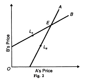
In this situation, the duopolists follow consistent behaviour patterns and the solution is determinate. This is illustrated in Figure 2 where the “variable” is interpreted as price. In this rival’s price increases. If A acting as the leader raises his price from L_B upward, В follows him by raising his price from L_A upward, so that both ultimately reach the equilibrium point E. Thus the solution is determinate.

(2) If ‘В’ desires to be a leader and ‘A’ a follower:

The solution is again determinate because both follow consistent behaviour patterns. This is again illustrated in Figure 2. Now В acts as the leader and A as the follower. When В raises his price from L_K upward, A follows him by raising his price from L_B upward, till both reach the equilibrium point E. Thus the solution is again determinate.

(3) If both A and В desire to be leaders:

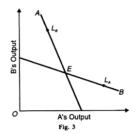
Each assumes that the behaviour of the other is governed by his reaction function. But, as a matter of fact, neither follows the reaction function of the other. Thus there is no equilibrium situation. This is known as the “Stackelberg disequilibrium”. This is illustrated in Figure 3 where the ‘variable’ is interpreted as the quantity of output. Each seller suffers from the rise in the output of his rival.

The profit maximisation output of one seller falls when his rival’s output increases. If В acts as the leader and increases his output from L_A onward, the reaction on A would be to reduce his output from L_B downward. But A does not follows В because he also considers himself a leader and so does not reduce his output from L_B downward. So there is no possibility of equilibrium at point E. This is the Stackelberg disequilibrium.

(4) If both A and В desire to be followers:

There is a determinate solution because each acts as a follower knowing that the other will also act as a follower. Suppose in Figure 2 seller В thinks that seller A has raised the price of his product, so В will follow him by raising the price of his product.

Now it is A’s turn to follow В in raising the price of his product. Then В will follow him and so on till both reach the equilibrium point E. Thus the followership solution is determinate.

Its Criticism:

The Stackelberg solution successfully links the duopoly problem to a family of related market structures. But “the theory is developed around the use of reaction functions expressing individual profit maximisation for given values of the rival’s variable.” This limits the use of the theory by excluding the problem of collusion and co-ordination among duopolists.

1. The exclusion of the problem of collusion has led to unrealistic results. No doubt the leadership equilibria (cases 1 and 2) contain an element of collusion or of spontaneous coordination, yet they represent an arbitrary form of coordination when leadership expresses itself in selecting a point along a reaction curve of the traditional kind.

Such leadership equilibria carry little meaning in relation to joint profit maximisation.

2. Even the intersection-point equilibria rest on arbitrary and wrong notions regarding the behaviour of the rival seller. They are based on the assumption that the value of the rival’s variable is given regardless of the seller’s own moves. The intersection-point equilibria result from a mutual attempt to follow the rival’s leadership. But the point selected on the reaction function by one seller does not play any part in shaping the policies of the rival seller. Thus the assumption on which this analysis is based is arbitrary and incorrect.

3. The Stackerlberg disequilibrium which results from the attempts at leadership on the part of both the sellers is also based on wrong reasoning and arbitrary assumptions. It may result from the assumption that the rival seller moves along a reaction curve which, in reality, does not exist for him. Or, it may result from the argument that the rival seller is forced into reacting along a curve which does not exist for him and thus to force him to act as the follower.

Thus the reaction curves of the Stackelberg solution, based as they are on conjectures, have made his theory weak and unrealistic. Despite these weaknesses, the Stackelberg model shows the importance of mutual interdependence between duopolists. If they recognise it, they will be able to earn profits, and if they ignore it both will be losers. If they enter into a collusive agreement, they may maximise their profits jointly.

Duopoly Model # 3. The Chamberlin Model:

Prof. Chamberlin proposed a stable duopoly solution recognising mutual dependence between the two sellers. He criticised and rejected both the Cournot and Bertrand cases on the ground that none of them conforms perfectly to the hypothesis that each seller acts so as to render his profit a maximum. In order to do this, a seller will take account of his total influence upon the price, indirect as well as direct.

When a seller remains passive to changes in price or output of his rival, it is a direct influence. On the other hand, when a seller reacts to the price or output changes of his rival and changes his own price or output, the influence in indirect.

According to Chamberlin, when interdependence is recognised between sellers, both direct and indirect influences of a change in the price or output of a seller lead to a stable industry equilibrium with monopoly price and output.

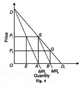
The Chamberlin solution can be explained both in terms of output adjustment and price adjustment. Let us take Figure 4 where seller A enters the market as a monopolist first, as in the Cournot model and maximises his profit by selling OA output at OP₁ price, thereby earning OASP₁ monopoly profit. Seller В enters the market after him and considers SD₁ segment of the market demand curve (DD₁) as his demand curve.

Under the Cournot assumption that his rival A will not change his output, he will sell AB output at OP₂ (=BG) price. The difference arises in Chamberlin’s solution from this point. In the Cournot model, each rival acts independently. But Chamberlin assumes their interdependence. So seller A does not react to B’s move and compromises with the existence of B.

Accordingly, he decides to reduce his output from OA to OE equal to B’s output AB. Seller В also recognises interdependence and realizes that by selling EA output at a higher price OP₁ he will share the monopoly profit.

Thus by recognising their interdependence, each seller shares equally the monopoly industry output OA, seller A selling OE and seller В selling EA. They also share the total monopoly profit OASP₁ equally between them, A earning OEKP₁ and В earning EASK at the monopoly price OP₁. Thus OP₁ (=AS) is a perfectly stable price, because either seller can bring disaster upon himself as well as upon his rival by behaving differently.

Chamberlin also shows that the result would be identical if sellers adjust their prices rather than their supplies. Suppose the price is anywhere between OP₁ and OP₂ In order to earn maximum profit, if A increases his price to OP₁. В will at once follow suit.

Thus В also raises his price to OP₁ to get the maximum possible profit. Once the price OP₁, is set, no one will cut it, for each seller realizes that by so doing, he will reduce his profit. The equilibrium is again stable and determinate.

The Chamberlin solution involves a kind of agreement between the two sellers. They do not sign it, but each seller is intelligent enough to realise the importance of mutual dependence. Each act rationally, looks beyond his nose and understands that sharing monopoly profit is to the best of his advantage.

Thus in Chamberlin’s model the sellers are independent, yet they are in a kind of collusion which leads to stable equilibrium, a sort of monopoly equilibrium.

Its Criticism:

The Chamberlin model is not free from certain weaknesses:

1. Like the Cournot and Bertrand models, it ignores entry of firms and is thus a closed model.

2. This model involves joint-profit sharing with zero enforcement costs by rivals. But problems might arise in sharing profit by the two sellers.

3. Fellner does not agree with Chamberlin that monopoly solution is possible under duopoly interdependence. A firm often underestimates the elasticity of the market demand curve and overestimates the elasticity of its own demand curve.

The underestimation of the market demand curve leads to the wrong estimation of the market MR curve. This may lead the collusive firms to charge a price higher than the monopoly price. A high price yielding very high profits may lead to the entry of firms into the industry; thereby make the Chamberlin solution impossibility.