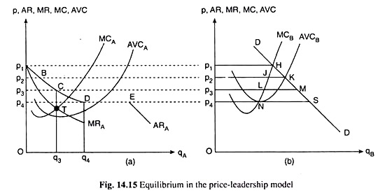
In the price-leadership model, there is one dominant firm in the industry that fixes up the price of the product and all other firms accept that price and determine their quantities accordingly.
The simplest case of price leadership under the following assumptions:
(i) There are two independent firms,
(ii) They produce perfect substitute products,
ADVERTISEMENTS:
(iii) The product is pershiable so that it must be sold within the period,
(iv) There are many knowledgeable buyers of the product,
(v) Each duopolist knows the market demand curve for the product,
(vi) The goal of each firm is profit maximisation in each period,
ADVERTISEMENTS:
(vii) The duopolist A assumes that B will always charge the same price as he (A) fixes, and B actually does this, i.e., here duopolist A is the price-leader and B the price-follower. We may now explain the working of the model with the help of Fig. 14.15.
In Fig. 14.15(b), DD is the demand curve for the product, and MCB and AVCB are the marginal and average variable cost curves, respectively, of duopolist B, the price-follower, and in Fig. 14.15(a), MCA and AVCA are the marginal and average variable cost curves of duopolist A, the price-leader.
Now, at each price that A fixes and B accepts, B will produce and sell his profit-maximising quantity and A will produce the quantity which is equal to the difference between the demand for the product at the price fixed by A and the quantity produced and sold by B, provided this difference is positive.
ADVERTISEMENTS:
For example, if A fixes the price at Op1 per unit, B will accept that price as exogenously given and will produce and sell the quantity p1H per period. This is his profit- maximising quantity because at this quantity his MC becomes equal to the price (i.e., Op1).
Now, as is seen in Fig. 14.15(b), p1 is equal to market demand at p = Op1. Therefore, nothing of the market is left for duopolist A at p = Op1. So at this price, A’s output would be equal to zero, and the point p1 on the vertical axis in Fig. 14.15(a) becomes a point on the demand curve of duopolist A.
Similarly, at the prices Op2, Op3 and Op4, duopolist B’s profit-maximising outputs would be p2J, p3L and p4N, respectively, and, as A accepts these positions, he would be able to sell at these prices, the quantities JK, LM and NS, respectively.
These quantities are equal to p2B, p3C and p4D in Fig. 14.15(a), i.e., at the prices Op2, Op3 and Op4, duopolist A would be able to sell the quantities p2B, p3C and p4D. Therefore, the points B, C and D, as also the point p1, would lie on the demand curve of duopolist A, and so his demand curve would be obtained to be the curve p1BCD.
But this is one segment of the curve. At the price Op4, there would be a discontinuity in the demand curve of duopolist A. This is because Op4 is equal to AVCB and, if the price falls below Op4, duopolist B’s output would be reduced to zero, as he would not be able to recover even the variable costs in the short run.
Therefore, for p < Op4, the market demand curve itself would be the demand curve of duopolist A. To be more specific, the demand curve of duopolist A is a curve in two parts—for p > Op4, his demand curve would be the segment p1BCD; at p = Op4, there would be a discontinuity—from the point D to the point E—in the demand curve; and at p < Op4, the market demand curve itself would be his demand curve or AR curve—this segment of the demand curve is EARA.
Therefore, obtained the demand curve of the price-leader, i.e., duopolist A. Now, the curve MRA in Fig. 14.15(a) is a segment of the MR curve of A for q < p4D = Oq4,—this curve bears the AR-MR relation with duopolist A’s AR curve. Given the MRA and MCA curves, we may immediately spot the equilibrium point of the price-leader, i.e., duopolist A, to be the point T in Fig. 14.15(a).
This point which is the point of intersection of the MRA and MCA curves, shows A that he should set the price of the product at Op3.
As the price-leader A sets the price at Op3, the follower, i.e., duopolist B, would accept the price and, at this price, his profit-maximising output would be p3L in Fig. 14.15(b). His profit-maximising price-output combination, therefore, would be (Op3, p3L) at the point L, and duopolist A would be left with the residual portion of market demand at p = Op3.
ADVERTISEMENTS:
This portion is LM in Fig. 14.15(b), or, p3C = Oq3 in Fig. 14.15(a). Duopolist A, then, would settle at the point C (p = Op3, q = Oq3) on his demand curve. Since at the price-demand combination, C (Op3, Oq3), duopolist A’s MR has been equal to his MC, he would be able to maximise profit at this combination, or, he would be in equilibrium if he sells Oq3 of output at the price of Op3.
The simple model that we have discussed above helps us to understand the economics of price leadership. More complicated models may be built up by increasing the number of firms, by introducing product differentiation or by varying the relationship between the cost curves of different firms. But they would not add much to economics of price leadership.
If in an oligopolistic industry, there is a large firm and a few small firms, then it is very probable that the large firm will successfully impose some sort of price leadership on the smaller firms. It may be the result of a tacit agreement. However, if the oligopolists are more or less of the same size, then the leadership agreement is likely to be based on firmer foundations than tacit acceptance.
