Robert Solow’s Neo-Classical Economic Growth Model

Let us make an in-depth study of the Robert Solow’s Neo-Classical Economic Growth Model:- 1. Assumptions of the Solow’s Model 2. The Solow Model 3. Possible Growth Patterns 4. Path of Divergence 5. Theoretical and Practical Importance of the Solow’s Model 6. Criticism of the Solow’s Model.

Assumptions of the Solow’s Model:

Solow’s model of growth is based on the following assumptions:

(i) A single composite commodity is produced.

(ii) Law of constant returns to scale operates i.e., the production function is homogeneous of first degree.

(iii) There are only two factors of production—labour and capital—which are paid according to their marginal productivity.

(iv) The output produced is regarded as net output i.e. proper allowance for the depreciation of capital is made.

(v) A flexible system of price-wage-interest prevails. This assumption plays an important part in the neo-classical adjustment process.

(vi) Technical neutrality is assumed i.e. technical progress does not influence the productivity of capital and efficiency of labour.

(vii)There is full-employment of labour.

(viii) The available capital stock is fully utilised.

(ix) Limited substitutability between capital and labour exists.

In addition to these assumptions, Solow assumed perfect foresight for all entrepreneurs and individual investors and smooth adjustment in goods, labour and capital markets. These imply that saving and investment plans are simultaneously fulfilled and that neither miscalculated output nor misdirected investment can ever arise. Market clearance is usually achieved (i.e. operation of Say’s Law is valid) and Keynesian unemployment is hardly possible.

The Solow Model:

Solow’s model of growth can be explained in a simple, non-mathematical way, even though he has himself given a mathematical exposition. We start with the introduction and then go to the mathematical treatment of his model. Having given the assumptions of Solow’s model, now we turn to the mathematical analysis.

The model assumes the production of a single composite commodity in the economy. Its rate of production is denoted by sY(t) which also represents the real income of the community. Part of the real income is consumed and the rest is saved and invested.

The proportion of the real income saved is denoted by s and it is regarded as constant. Thus the rate of saving would be sY(t), i.e., the product of propensity to save and the real income The community’s stock of capital in “t” period of time is denoted by K(t) and it takes the form of accumulation of the composite commodity. Net investment refers to the rate of increase in capital stock and is denoted by dK/dt or K^t. So the basic identity between saving and investment can be expressed as

K^t = sY …(1)

The production function representing the various technological possibilities can be expressed as

Y = F (K, L) …(2)

where Y refers to real output, F stands for functional relationship, K and L represent the factors capital and labour respectively. Substituting the value of Y in (1) we get

K^t= sF(K, L) …(3)

where K^t is the stock of real capital at the point of time t.

This equation (3) contains two unknown quantities. We need to know demand for and supply of labour as well as capital so that we can find out the equilibrium value of the capital-output ratio. One way to close the system would be to add a demand-for-Iabour function showing that marginal physical productivity of labour equals real wage rate and another relation can be supply-of-labour equation. The latter can take the general form of making labour supply a function of real wage (W). For solution, there should be three equations for three unknown variables K, L, W.

Equation (3) represents the supply side of the system. Now we have to spell out the demand side of the system too. Solow’s demand side of the system is obtained from the supply of labour to the economic system being offered for employment which influences the wage rate and hence the capital intensity of production.

Solow has written the supply of labour in the following form:

L(t) = K₀e^nt … (4)

This relation tells that supply of labour L_(t) is equal to the number of labourers who offer for employment. As population growth is the result of exogenous factors, so the assumption is that labour force increases at a constant relative rate n. Assuming technical neutrality, n represents Harrod’s natural growth rate. The right hand side of equation (4) shows that the labour force increases at the compound rate (n) from period o to period t.

Relation (4) can also be explained in another way. This relation can be viewed as a supply curve of labour. It says that labour force grows at an exponential rate (n) and its supply curve at a particular time is completely inelastic because full- employment is assumed to be perpetually maintained.

In other words, the labour supply curve is a vertical line which shifts to the right as the labour force available for employment increases. Then the real wage rate adjusts so that all available labour force is employed. The real wage rate (w) is determined by the equality of marginal wage with marginal productivity and it is expressed as

W =dF(K,L)/dL

With the introduction of marginal productivity equation written above, Solow’s system is complete one, as there are 3 unknowns and three equations. Substituting the value of L(t) in equation (3), we get the following relation

K^t = sF(K, L₀e^nt) …(5)

Solow regards this as the basic equation for his growth model because it helps in determining at any time the volume of capital stock needed to provide employment to all the available labourers. In other words, the solution of this equation gives the time profile of growth of the community’s capital stock which would fully employ the available labour.

Once we know the time path of capital growth and that, of the labour force, i.e. K and L, we can compute from the production function the corresponding time path of real output. The time path of real wage rate (w) is determined by the marginal productivity equation written earlier.

Prof. Solow has summed up his argument as follows: “At any moment of time, the available labour supply is given by equation (4) and the available stock of capital is also a datum. Since the real return to factors will adjust to bring about full employment of labour and capital, we can use the production function of equation (2) to find out the current rate of output. Then the propensity to save tells us how much of net output will be saved and invested. Thereby we know the net accumulation of capital during the current period. Added to the already accumulated stock this gives the capital available for the next period and the whole process can be repeated.”

Possible Growth Patterns:

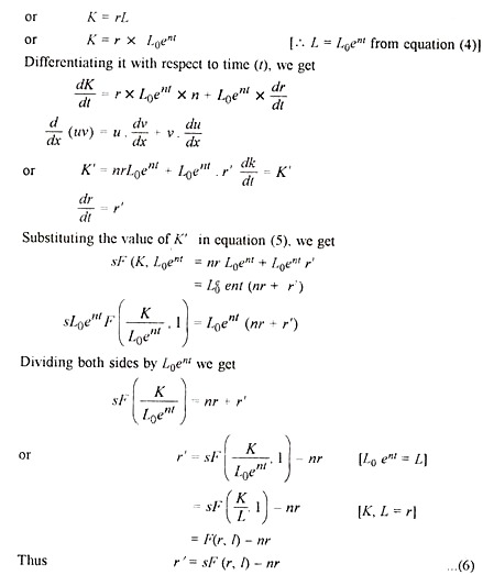
In order to observe whether a particular rate of capital accumulation is always consistent with the given growth rate of labour force, we must study the growth equation (5) for the qualitative nature of its solutions. We know that without specifying the exact shape of the production function, we cannot hope to find out the steady state solution. To do so Solow has introduced a new variable, the capital- labour ratio, r

Equation (6) is the fundamental equation which can be used for illustrating the various growth patterns. In this equation, r is the capital-labour ratio (K/L), n is the relative rate of change in labour force (L’IL), F(r, l) represents output per worker.

In other words, SF(r, I) is the total product curve showing the various levels of output when various capital-labour ratios (r) are employed with one unit of labour. Equation (6) clearly shows that the rate of change of capital-labour ratio (r’) is the difference of the two terms SF(r, I) and nr.

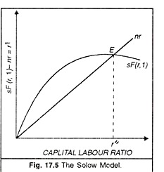
In Fig. 17.5, capital-labour ratio is shown on the horizontal-axis and the difference between sF(r I) and nr is shown on the vertical axis. The ray drawn through the origin with slope n represents the function nr. The total productivity curve is the function of sF(r, I). This curve is passing through the origin and is convex in shape. The convexity of the curve represents diminishing marginal productivity of capital. E is the point of intersection of the ray nr and the curve sF(r, I). At this point of intersection nr = sF(r, I) and r” = 0. When r”- o, the capital-labour ratio would be constant and the stock of capital would expand at the same rate as the labour force i.e. n.

Once the capital-labour ratio r” (i.e. the capital- labour ratio in the equilibrium position) is established, it will be maintained, as capital and labour will grow in the same proportion. Because of the operation of constant returns to scale, the real output will also grow at the same relative rate n, and output per head of labour force (i.e. average productivity of labour) will also be constant. So E is the point of steady growth and r “is the desired capital-labour ratio which can maintain the steady growth.

Path of Divergence:

Now we study the behaviour of capital-labour ratio if there is a divergence between r and r”.

There are two possibilities:

(i) When r > r”

(ii) when r < r”

Take the first possibility when r > r “, this can occur when the economy happens to be to the right of the equilibrium point E. Under this situation nr > sF (r, 1) and from equation (6) we can see that as r moves towards r “equilibrium will be established again at E and steady growth would be maintained. On the opposite, when r < r” this can occur to the left of intersection point E. Under this situation, nr < sF (r, I) and r will move towards r”.

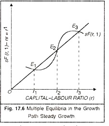
Equilibrium will again be established at point E and steady growth will be maintained. Thus the equilibrium value of r” is stable. The instability of the Harrod-Domar model is gone. Prof. Solow has summed up the discussion thus: “whatever the initial value of the capital-labour ratio, the system will develop towards a state of balanced growth at the natural rate. The time path of capital and output will not be exactly exponential except asymptotically. If the initial capital stock is below the equilibrium ratio, capital and output will grow at a faster pace than the labour force until equilibrium value is approached. If the initial ratio is above the equilibrium rate, capital and output will grow more slowly than the labour force. The growth of output is always intermediate between those of labour and capital.” But it should be understood that the stability position shown in Figure 17.5 is not inevitable. It all depends upon the shape of the productivity curve sF(r, I). This point is illustrated with the help of Figure 17.6, In this figure, the productivity curve sF(r, I) intersects the ray nr at three different points E₁ E₂ and E₃. Corresponding to these three points of intersection the capital-labour ratios are r₁ r₂ and r₃.

Inspection of these points shows that E₁ and E₃ are the stable equilibrium while E₂ is an unstable equilibrium because production curve sF(r, I) is intersecting nr from above. E₂ is a point of unstable equilibrium because the production curve is intersecting nr from below. Let us now discuss as to how the stable equilibrium is maintained. Suppose the initial capital- labour ratio is less than r₂ (i.e. anywhere between r, and r₂), the system will revert to the equilibrium at a low capital-labour ratio i.e. r₁.

Correspondingly the rate of increase of output will be low. On the contrary, if the initial capital-labour-ratio is more than r₂ (i.e. anywhere between r₂ and r₃), then the system will move forward and would ensure the cumulative growth and equilibrium will be established at a higher capital-labour ratio i.e. r₃.

Prof Solow has observed in this connection:

“The relevant balanced growth equilibrium is at r, for any initial ratio anywhere between o and r₂; it is at r₃ for any initial ratio greater than r₃. The ratio r₂ is itself an equilibrium growth ratio but an unstable one; any accidental disturbance will be magnified over lime.”

The main conclusion of Solow’s analysis is that “when production takes place under the usual neo-classical conditions of variable proportions and constant returns to scale, no simple proposition between natural and warranted rates of growth is possible. There may not be any knife-edge. The systems can adjust to any given rate of growth of labour force and eventually approach a state of steady proportional expansion.”

Theoretical and Practical Importance of the Solow’s Model:

Solow model is neo-classical in character, and it is evident from Solow’s own comments: “I have been deliberately as neo-classical as you can get.” Solow’s model is a synthesis of the classical and modern views. This model retains the basic assumptions of the classical model i.e., existence of full employment and perfect competition etc. and removes the difficulties and rigidities associated with the post- Keynesian growth analysis. Thus, it is a full-employment model which at the same time attempts to maintain the conditions of steady growth.

The model has its practical importance. It seeks to maintain full-employment through choice of the appropriate technique. The various routes to full-employment via fiscal, monetary and population policies, leaves the nation some leeway to choose whether it wants high employment with high capital investment (rapid growth and low consumption) or the reverse or some mixture of both. An important advantage of this model of growth is that it provides a theoretical apparatus of exploring these practical possibilities.

Criticism of the Solow’s Model:

The objections raised against the Solow model over the years have to be classified into three categories represented by the Modern Cambridge School, Ryuzo Sato, and Robert Eisner.

1. The Modern Cambridge School. This school comprises of economists notably Mrs. Robinson, Kaldor and Pasinetti. These economists attacked the realism of Solow’s assumptions. The main objection against Solow’s model has been its empirical validity.

The Cambridge economists mention the following objections specifically:

(a) There is no investment function which depends upon profit rate.

(b) The theory does not explain the pace and direction of technical progress.

(c) The marginal productivity theory of distribution (basis of Solow theory) is “all non-sense”. It is suggested that marginal productivity theory of distribution should be replaced by “a Keynesian theory of distribution”.

(d) The theory assumes variable capital-labour ratio. But for one thing, capital labour ratios are often fixed by technology. Eleven men can hardly share ten spades

(e) The separation of technical progress and capital deepening as done by Solow is rather tenuons, since the two are interdependent.

2. Ryuzo Sato contends that variation of the capital-labour ratio in reality cannot be possibly very wide. He, therefore, believed that the Harrod-Domar rigidity in factor-proportions is essentially correct. But empirical studies reveal that such objections about the nature of production function are relatively unimportant.

3. Robert Eisner criticised the Solow’ analysis. In his view, Solow did not pay adequate attention to the Keynesian difficulties, e.g., liquidity traps, downward inflexibility of wage rate, etc. Moreover, marginal product of capital may become zero at some finite capital-labour ratio. Therefore, Solow’s analysis too has limited empirical validity.

Conclusion:

Though this model suffers from some weaknesses, yet its importance cannot be minimised. The major contribution of this model is to establish the automatic stability of neo-classical growth path through the market adjustment mechanism. The major attraction of this model lies in its sweep and simplicity. Solow’s model has been a major landmark in the history of growth economics in that it opened up the discussion of technical progress into growth models of the neo-classical variety.