Effectiveness of Monetary Policy in India (With Diagram)

Let’s study the effectiveness monetary policy in influencing income (na­tional) and interest rate.

Quantity theory of money as suggested by the classical authors states that money supply is directly propor­tional to the level of aggregate demand (as­suming velocity of money is constant).

This means that money supply does not affect the demand for money demand as a fraction of total spending remains stable.

But, this classical notion is not convincing monetary expansion indeed affects demand for money. Once monetary policy is employed interest rates are then influenced. A tight mon­etary policy means a rise in the interest rate while expansive monetary policy pushes in­terest rate down. Demand for money is then affected by the interest rate. Or demand for money (both transaction and speculative) is responsive to changes in the rate of interest.

We will now discuss the rela­tion between money supply growth and de­mand for money again in terms of IS-LM model.

We know that the point of intersection of the IS and LM curves gives us the equilibrium combinations of income level and the rate of interest. This is a situa­tion of simultaneous equilibrium of both prod­uct market and money market. We call it also a situation of general equilibrium. There we did not make any specific reference to the elasticities of either the IS function or the LM function.

If these elasticities are taken into ac­count, our previous conclusions need to be modified and qualified. However, we won’t consider here elasticity of IS schedule. Since we are interested in knowing the effectiveness of monetary policy, we will deal even some extreme cases of elasticity of the LM function.

Monetary policy aims at achieving the macroeconomic policy objectives through the control over money supply. The slope of the LM curve depends on the interest elasticity of money demand. If the interest elasticity of money demand is assumed to be high, the LM curve will be relatively flat.

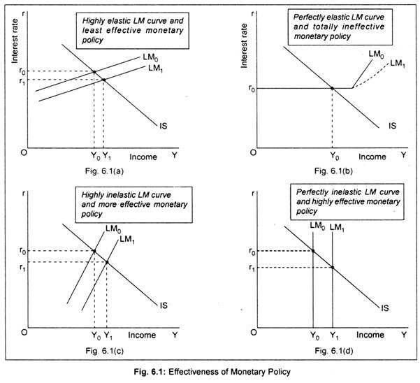
On the other hand, LM curve becomes relatively steep if the in­terest elasticity of money demand becomes low. Let us consider two extreme cases: (i) if interest elasticity of money demand is per­fectly elastic (i.e., liquidity trap), the LM curve becomes horizontal, and (ii) if the interest elas­ticity of money demand is zero, the LM curve becomes vertical. Consequences of an increase in money supply on interest rate and national income have been shown in Fig. 6.1.

It is seen from Fig. 6.1 that the initial equi­librium interest rate and income combination is r₀-Y₀ in all the figures. Further, the effect of an increase in money supply has been shown by the shifting of the LM curve from LM₀ to LM₁ in the rightward direction.

In Fig. 6.1(a) we have assumed a high in­terest elasticity of money demand causing the LM curve to become relatively flat. Following an expansion in money supply, interest rate declines marginally from Or₀ to Or₁ and in­come, too, rises insignificantly from OY₀ to OY₁. The fact is that monetary policy is leas¹ effective. The reason is: An increase in money supply at the initial level means an excess money supply over money demand. This then causes interest rate to fall. A fall in interest rate by a very small amount causes investment to rise by a very small amount making multiplier principle near-inoperative. That is why— national income rises by a very small amount.

Since money demand is highly elastic people hold liquid money for speculative purposes, invest less in securities and economise less on transaction purposes. All these suggest that monetary policy is least effective.

An extreme situation of perfectly elastic money demand has been considered in Fig. 6.1(b) that makes the LM curve perfectly elas­tic. This is called the Keynesian range of LM curve or the liquidity trap region. In this re­gion, an increase in money supply does not produce any effect either on interest rate or on income level. This is because at this floor rate of interest, security-holders exchange all their securities for liquid cash and, thus, all liquid cash gets trapped in this region. Any increase in money supply from LM₀ to LM₁ won’t make any impact on interest and in­come. This means that monetary policy is to­tally ineffective.

In Fig. 6.1(c) since interest elasticity of money demand is lower, an increase in money supply from LM₀ to LM₁ will result in a larger drop in interest rate as compared to Fig. 6.10 (a). As a consequence, multiplier effect will be stronger causing income level to rise by a greater amount.

Here the fall in speculative interest rate does not have much influence on money demand since in this case money de­mand depends on interest rate very little. An increase in money supply causes transaction balances to go up and speculative balances to go down as interest rate falls. This means monetary policy is highly effective.

An extreme situation of perfectly inelastic money demand may be explained in terms of Fig. 6.1(d). In contrast to the’ result of Fig. 6.1(b), an increase in money supply now causes a greater fall in interest rate and conse­quently a larger increase in income. This re­gion is called the classical region. In this re­gion, since interest rate is pretty high, money is demanded for transaction purposes only while speculative balances are nil.

Since no­body holds idle cash, an increase in money supply means fall in interest rate and a rise in income by a very bigger amount. This means monetary policy is highly or most effective in this range of LM curve.