Hicks-Hansen Theory | Economics

The two economists after Keynes, J. R. Hicks (1904-1989) and Alvin Hansen (1887-1975), have shown that although both the classical and _r Keynesian theories of interest are indeterminate, they together may give us a complete and determinate theory of interest. The theory of Hicks and Hansen, made up of these two theories, is known as the Hicks-Hansen theory of interest.

Classical Interest Theory and the IS Curve:

The equations of the classical theory of interest are:

s = s(r), s’> 0                      [eq. (17.1)]

i = i (r), i’ < 0                      [eq. (17.2)]

and s (r) = i (r)                  [eq. (17.3)]

where the meanings of the symbols are already known to us.

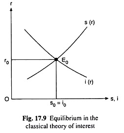
The equilibrium values of r, s and i that can be obtained by solving these three equations may also be obtained from Fig. 17.9 which is the same as Fig. 17.1. These values are, respectively, r₀, s₀ and i₀.

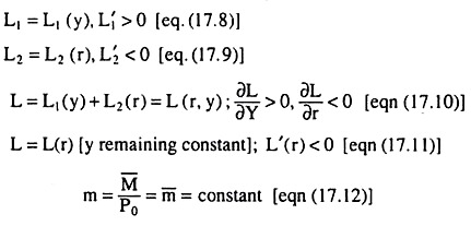
It has been assumed in this theory that saving (s) is a function of the rate of interest (r) only.

However, according to Keynes, apart from r, saving is also an increasing function of income (y). Therefore, following Keynes, we have

s = s(r, y); ∂s/∂r > 0, ∂s/∂y > 0                               [eq. (17.4)].

However, Keynes did not carry this idea to its logical conclusion. He only used it to argue that the classical theory was indeterminate. It was left to Hicks and Hansen to work further on this idea. They said that eqn. (17.4) was not an s curve only. It was a family of s curves.

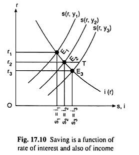
Accord­ing to them, since s = s(r, y), the position of the s (r) curve depends on the value of y. For each particular value of y, we have a separate s(r) curve. For y = y₁, y₂, y₃, etc. (…. y₃ > y₂ > y₁), the s curves in (r, s) space that we would obtain are s(r, y₁), s(r, y₂), s(r, y₃), etc.

These curves have been shown in Fig. 17.10. Since y₂ > y₁ and s is an increasing function of y, we would have at any r, s(r, y₂) > s(r, y₁), i.e., the s(r, y₂) curve lies to the right of the s(r, y₁) curve. Similarly, since y₃ > y₂, the curve s(r, y₃) would lie to the right of the curve s(r, y₂). In other words, as y rises, the s(r, y) curve would shift to the right.

If we now superimpose the i(r) curve on the family of s(r) curves in Fig. 17.10, we would get not a unique equilibrium value of r, but a number of such values one for each s(r, y) curve at the point of intersection of this curve with the i(r) curve. This gives us the indeterminacy of the classical theory. In Fig. 17.10, we see that, if y = y₁, the equilibrium r would be r₁ at the point of intersection of the s(r, y₁) and i(r) curves.

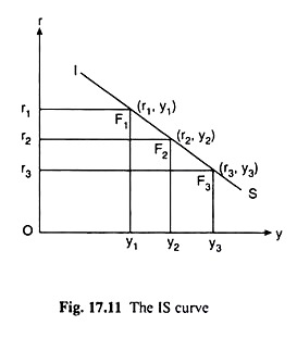
Similarly, if y = y₂ or y₃, the equilibrium values of r would be r₂ or r₃. That is, here we do not obtain any unique value of r; rather, we get different (r, y) combinations, viz., (r₁, y₁), (r₂, y₂), (r₃, y₃), etc. Let us now plot these combina­tions as points in the (r, y) space of a separate diagram, in Fig. 17.11. Now, the curve that is obtained by joining these points is known as the Hicks-Hansen IS curve. In Fig. 17.11

We have obtained the IS curve corresponding to the (r, y) equilibrium combinations of Fig. 17.10. At each point or (r, y) combination on the IS curve we have i(r) = s(r, y). That is why the curve is called an IS curve, and that is why the equation of the curve is

s(r, y) = i (r)                                         (17.14)

Since (17.14) is an equation in two unknowns, viz., rand y, it cannot be uniquely solved for either r or y; rather, we would obtain different (r, y) combinations as its solution. Let us also note that there is a one-to-one correspondence between the equilibrium points, viz., E₁, E₂, E₃, etc. in Fig. 17.10 and the points on the IS curve, viz., F₁, F₂, F₃, etc., respectively, in Fig. 17.11.

The Slope of the IS Curve:

The slope of the IS curve would be negative, i.e., it would be sloping downward towards right. This is because, as we see in Fig. 17.10, as y increases from y₂ to y₃ at any i = s point, E₂, the s(r, y) curve shifts to the right, from s(r, y₂) to s(r, y₃) and the point of intersection between the s and i curves moves downward towards right along the i(r) curve from E₂ to E₃ giving us a lower r, viz., r₃.

From the point of view of economics, we have this to say: As y increases at E₂, the s(r, y) curve shifts to the right.

Therefore, at the initial (equilibrium) r = r₂, s becomes greater than i(r₂T > r₂E₂). In the competitive capital market r now would be falling till at some rate of interest, s, falling along the new s(r, y) curve from the point T to E₃, and i, rising along i(r) curve from the point E₂ to E₃, would become equal to each other, and the market would come back to equilibrium at a lower r (viz., r₃) and a higher y (viz., y₃).

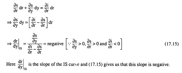
Therefore, along the IS curve, in Fig. 17.11, as y rises from y₂ to y₃, r would fall from r₂ to r₃, giving us the slope of the curve to be negative. We may also show with the help of calculus that the slope of the IS curve is negative. Taking total differential of (17.14), we have

 

 

 

 

 

 

 

 

 

Liquidity Preference Theory of Keynes and the LM Curve:

The equations of Keynes’ liquidity preference theory are

and L(r) = m̅                              [eqn. (17.13)]

where the meanings of the symbols are already known to us.

As we know, eq. (17.13) is the money market equilibrium condition. If other things, espe­cially, the level of income (y), remain unchanged, then from (17.10), we obtain

L = L₁ (y̅) + L₂(r) = L(r, y̅) = L(r); ∂L/∂ < 0                    [eqn. (17.11)]

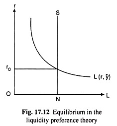
(17.11) is demand for money (L) curve in the liquidity preference theory—here L is a func­tion of r only. The equilibrium rate of interest is one at which the demand for money in real terms (L) becomes equal to the supply of money in real terms (m). Here the supply of money is taken to be an exogenously given con­stant (m = m̅). Therefore, at the equilibrium r, we obtain

L(r) = m̅                                   [eqn (17.13)].

Since there is only one variable, r, in (17.13), we may solve it for a unique value of r as we have done with the help of Fig. 17.6 or 17.12. The value of equilibrium r thus ob­tained is r = r₀ at the point of intersection of the demand for and supply of money curves, L(r, y̅) and NS, respec­tively.

It has been assumed here that L is a function of r only. But Keynes himself argued that the L₁ part of L is a function of y. That is why L is an increasing function y also, apart from it being a decreasing function of r owing to its L₂ part. All this we have represented in eqn (17.10).

However, Keynes did not carry this idea further. It was Profs. Hicks and Hansen who pointed out that (17.10) was not the equation of an L curve. It actually represented a family of L curves. They argued that since L = L (r, y), the position of the L (r) curve depends on the value of y. For each particular value of y, we have a separate L(r) curve.

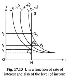
For y = y₁, y₂, y₃, etc. (… y₃ > y₂ > y₁), the L curves in (r, L) space that we would obtain are L(r, y₁), L(r, y₂), L(r, y₃), etc. These curves have been shown in Fig. 17.13. Since y₂ > y₁, and L is an increasing function of y, we would have, at any r, L(r, y₂) > L(r, y₁).

That is why the L(r, y₂) curve lies to the right of the L(r, y₁) curve. Similarly, since y₃ > y₂, the curve L(r, y₃) would lie to the right of the curve L(r, y₂). In other words, as y rises, the L(r, y) curve shifts to the right.

Let us now superimpose the supply of money curve NS on the family of L curves in Fig. 17.13. Since the sup­ply of money is assumed to be a constant, viz., m̅ = ON, the NS curve would be a vertical straight line. Here we would not get a unique equilibrium value of r, but a number of such values, one for each L(r, y) curve at its point of intersection with the NS curve.

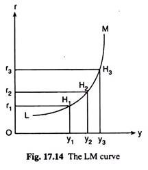
This gives us the indeterminacy of Keynes’ liquidity preference theory. In Fig. 17.13, we obtain that the equilibrium r would be r₁ at the point of intersection of the L(r, y₁) and NS curves. Similarly, if y = y₂ or y₃, the equilibrium values of r would be r₂ or r₃. That is, here we do not obtain any unique value of r; rather we get different (r, y) combina­tions, viz., (r₁, y₁), (r₂, y₂), (r₃, y₃), etc. Let us now plot these combinations as points in the (r, y) space of a separate diagram in Fig. 17.14.

Now, the curve that is obtained by joining these points is known as the Hicks-Hansen LM curve. In Fig. 17.14, we have obtained the LM curve corresponding to the (r, y) equilibrium combinations of Fig. 17.13.

At each point or (r, y) combination on the LM curve, we have L (r, y) = m̅. That is why the curve is called an LM curve, L and M standing for demand for money and supply of money (in real terms), and that is why the equation of the LM curve is

L(r, y) = m                                (17.16)

Since (17.16) is an equation in two unknowns, viz., rand y, it cannot be uniquely solved for either r or y; rather, we would obtain different (r, y) combinations as its solution. Let us also note here that there is a one-to-one correspondence between the equilibrium points G₁, G₂, G₃, etc. in Fig. 17.13 and the points on the LM curve, viz., H₁, H₂, H₃, etc., respectively, in Fig. 17.14.

The Slope of the LM Curve:

The slope of the LM curve would be positive corresponding to the negatively sloped seg­ment of the underlying liquidity preference (L) curve. This is because, as we see in Fig. 17.13, as y rises, at any L = M point, G₂, from y₂ to y₃, the L (r, y) curve shifts to the right from L (r, y₂) to L(r, y₃) and its point of intersection between the L and m̅ (here NS) curves, moves vertically upwards along the in curve [vertically, because the m̅ (or NS) curve here is a vertical straight line] from G₂ to G₃, giving us a higher r, viz., r₃. That is, _r as y rises, r also rises, giving us the positive slope of the LM curve.

As regards the economics behind this, we may say the following. As y increases at G₂, the L (r, y) curve shifts to the right. Therefore, at the initial equilibrium r = r₂, L becomes greater than m̅ (r₂V₂ > r₂G₂).

Consequently, people will sell bonds, and this will be followed by a fall in p_b and a rise in r. The rise in r will be followed by a fall in L along the higher L curve till, at some r = r₃, L would again become equal to m and the money market will come back to equilibrium at a higher r and a higher y.

Since the movement from the point G₂ to G₃ in Fig. 17.13 is the same as that from H₂ to H₃ along the LM curve in Fig. 17.14, and the point H₃ would have more of y and r than point H₂, we obtain that the LM curve is positively sloped. However, we should remember that the positive slope of the LM curve would be obtained if the slope of the L curve is negative.

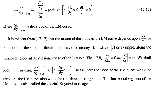
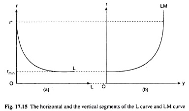
Of course, apart from the negatively sloped segment, the L curve would also have a vertical and a horizontal segment. We shall now see the LM curve also would be vertical or horizontal as the L curve assumes such shapes. Taking the total differential of (17.16), we have

 

  

Lastly, in the intermediate range of the L curve, we have – ∞ ∂r/∂L < 0, or, – ∞ < ∂L/∂r < 0. Here we get ∞ > dr/dy|_LM > 0, i.e., here the slope of the LM curve would be positive finite. Therefore, here the LM curve would be sloping upward towards right. This positively sloped segment of the LM curve is called its intermediate range.

Therefore, that like the L curve, the LM curve would also have a horizontal, a vertical and an intermediate range. We have also seen that both the L and the LM curves are horizontal at the same r which is r = r_min, and their vertical segments begin at the same r which is r = r*, and both the curves have their intermediate ranges at r_min ≤ r ≤ r*. All these points are observed in Figs. 17.15(a) and (b).

Determination of the Rate of Interest in Hicks-Hansen Theory:

The IS curve passes through the (r, y) combinations that satisfy the condition s(r, y) = i(r). This condition is the equilibrium condition in the capital market as also the equilibrium condition in the goods market.

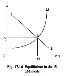
On the other hand, the LM curve passes through the (r, y) combinations that satisfy the condition L(r, y) = M (the money supply in real terms), which is the equilibrium condition in the money market. Therefore, the (r, y) combination that would be obtained at the point of intersection of these two curves (IS and LM), would give us simultaneously the equi­librium in the goods market and that in the money market.

In Fig. 17.16, E is the point of intersection of the IS and LM curves. At the point E, we obtain that if the economy’s level of income and the rate of interest be y₀ and r₀, then the goods market and the money market would be in equi­librium simultaneously.

Here the equilibrium in the goods market or equilibrium in the level of income cannot be dis­turbed by the lack of equilibrium in the money market giv­ing rise to a change in the rate of interest and in the level of investment.

Also, the equilibrium in the money market can­not be disturbed by the disequilibrium in the goods market leading to change in the level of income and the rate of interest.

Therefore, the Hicks-Hansen IS-LM theory is able to determine a unique equilibrium rate of interest (r₀ in Fig. 17.16) along with a unique equilibrium level of income (y₀ in Fig. 17.16). That is why the IS-LM theory may be considered to be a complete theory of interest rate determination.