Economic growth of a country is possible if the exact condition of the economy is determined.
Economic analysis is a process in which the strengths and weaknesses of an economy are determined.
It is a systematic approach to determine the optimum use of scarce resources, compare available alternatives, and select the best alternative to achieve a particular goal. In addition, economic analysis helps in determining the causes of various economic problems, such as inflation, depression, and economic instability.
Economic analysis is performed with the help of various tools, which are shown in Figure-1:
The different tools of economic analysis (as shown in Figure-1) are discussed in detailed below.
Economic Variables:
The main aim of economic analysis is to identify the nature of economic variables and determine the level of relationship between two or more related economic variables. An economic variable refers to the any economic quantity whose value changes with a change in its determinants or change in economic activities.
For example, demand, supply, prices, production cost, wages labor and capital are the economic variables whose value changes with change in their determinants or in different trade cycles. Most of the economic variables are related as well as dependent on each other. Therefore, a change in one economic variable brings changes in the value of other economic variables.
ADVERTISEMENTS:
Economic variables can be classified as follows:
(a) Dependent Variables:
Involve those variables whose values are dependent on the values of other variables. Moreover, the values of these variables are affected by change in the value of other interrelated variables.
For example, demand of a product is dependent on its price. This implies that demand of a product falls with increase in its prices and vice versa. Therefore, the demand of a product is a dependent variable.
ADVERTISEMENTS:
(b) Independent Variables:
Refer to variables that are independent and are not affected by a change in any other variable. In the preceding example of demand of a product and its price, the demand of the product is a dependent variable, while price of the product is an independent variable.
(c) Endogenous Variables:
Refer to variables whose value can be obtained within the model under consideration. For example, the price of a product in the supply and demand model is endogenous. This is because the price of the product is set in response to consumer demand.
(d) Exogenous Variables:
Refer to variables whose value is obtained outside the model under consideration. For example, in case of increase in domestic petrol price due to increase in international petrol price, the international petrol price is the exogenous variable.
Slope:
Slope is one of the most important tools used for economic analysis. It helps in determining the changes produced in one variable with a change in another variable. Therefore, slope can be defined as the change occurs in dependent variable due to the change in independent variable. The relationship between a dependent and independent variable can be represented as a straight line on a graph.
The shape of line determines the type of relationship between the two variables. This line is termed as the slope of line. If the slope is steeper, then the relationship between the two variables is weak and vice-versa. Suppose a unit change in the independent variable x brings changes in the dependent variable y.
ADVERTISEMENTS:
In such a case, the slope would be:
Slope = change in y/change in x
If the slope of a line is positive, the line moves upward when going from left to right. On the other hand, if the slope is negative, then the line moves down when going from left to right.
Let us understand the concept of slope with the help of an example. In demand curve, the slope represents the ratio of the change in the independent variable price (P) to the change in the dependent variable that is demand (D). If the price of a product decreases (- AP), then the demand for that product would increase (AD).
ADVERTISEMENTS:
In such a case, the slope of the demand curve would be as follows:
Slope = -∆P/∆D
Where, -∆P = change in price (independent variable)
∆D = change in demand variable (dependent variable)
ADVERTISEMENTS:
The slope differs for linear and non-linear variables.
Linear Function:
Let us understand linear function with the help of linear demand function.
Suppose the linear demand function is as follows:
Dx = 20 – 2Px
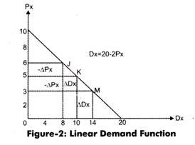
The demand curve for the preceding demand function is shown in Figure-2:
ADVERTISEMENTS:
In Figure-2, it can be noted that the slope of the curve changes. For example, when price (Px) = 3, then the demand (Dx) = 14. After that, the price increases to 5 and quantity demanded decreases to 10. In such a case, -∆P = 3-5 = -2 and ∆D = 14-10 = 4. Here negative sign indicates the inverse relationship between demand and price of a product.
Therefore, the slope of the demand curve is equal to:
Slope = ∆P/∆D
Slope = 2/4
Slope = 0.5
ADVERTISEMENTS:
Therefore, the slope between the points M and K is 0.5. Similarly, we can find out the slope between the points J and K. At point K. the price (Px) = 5 and demand (Dx) = 10. After that, the price increases to 6 and quantity decreases to 8. In such a case, -∆P = 5-6 = -1 and ∆D = 10-8 = 2.
Therefore, the slope of the demand curve is equal to:
Slopes = ∆P/∆D
Slope = 1/2
Slope = 0.5
The slope between the points J and K is 0.5. Now, it can be said that the slope is equal at all points in the linear demand function.
ADVERTISEMENTS:
Non-Linear Function:
Let us continue the example of demand function. In non-linear demand function, the slope of demand curve changes at every point. Therefore, the determination of slope in non-linear demand function can be performed by comparing the slope within and at a point on the demand curve.
The non-linear demand function can be given as follows:
Dx = 32Px-2 = 32/Px2
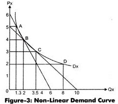
The demand curve for non-linear demand function is represented in Figure-3:
From Figure-3, let us determine the slope between A and B and C and D.
ADVERTISEMENTS:
The slope between A and B point is equal to:
Slope = ∆P/∆D
Slope = 4-5/2-1.3
Slope = -1.43
The slope between C and D point is equal to:
Slope = ∆P/∆D
Slope = 2-3/8-3.5
Slope = -0.23
The slope between the two sets A and B and C and D are different. This implies that the slope of nonlinear demand function would be different between two different sets of points.
In a nonlinear demand curve, the slope is different not only in between the points but also at every point. For example, the slope at point B and D on demand curve can be calculated by drawing a tangent from point B. The slope of tangent and demand curve is equal in measurement.
The slope of tangent or slope at point B is equal to:
Slope = ∆P/∆D
Slope = 0-6/6-0
Slope = -1
Therefore, slope at point B is 1. Similarly, we can draw a tangent from point C and calculate the slope of tangent or slope at point C of demand curve.
The slope at point C of demand curve can be determined as follows:
Slope = ∆P/∆D
Slope = 0-4.5/10-0
Slope = -4.5/10
Therefore, the slope at point C of demand curve is equal to -4.5/10.
This method of slope determination has certain limitations, which are as follows:
a. Lacks reliability because difference in the slope of a demand curve can produce a larger change in the independent variable. For example, the slope between two points A and D is -0.44 but the slope between the points that lie in between these two points is large, B and C is -0.66. Therefore, it is not a proper method for the determination of slope.
b. Fails to determine the solution for an optimization problem because it involves polynomial functions.
Due to aforementioned limitations of the method, another method, differential calculus is used for determining the slope at a point in the demand curve.
The demand function used for the determination of slope at a point with the help of differential calculus is as follows:
Dx = 32Px-2
For the calculation of slope by differential calculus, we need to first take the first derivative of demand function as follows:
∂D/∂P = (-2) 32Px-3 = -64/Px3
Taking the reciprocal of the preceding equation, we get
∂P/∂D = -Px3/64
With the help of the preceding equation, we can determine the slope of any point in the demand curve.
For example, at point B, the slope of demand curve can be calculated as follows:
∂P/∂D = – (4)3/64
∂P/∂D = -1
Therefore, the slope at point B of demand curve is -1 as it was calculated with the tangent method.
Differential Calculus:
In above, we have used the differential calculus method for measuring the slope of a demand curve. Differential calculus provides an optimum solution for economic problems and supports decision-making. For understanding the concept of differential calculus, we first need to get acquainted with the basic rules of differential calculus. Let us first understand the concept of derivative. Derivative can be explained with the help of Marginal Cost (MC), which refers to a change occurred in the Total Cost (TC) due to a unit change in total output (Q).
The formula used for the calculation of MC is as follows:
MC = Change in TC/Change in Q
Or MC = ∆TC/∆Q
The value of ∆Q is assumed to be one. The aforementioned equation cannot be used when the value of ∆Q is very small as it tends to be zero. This problem can be overcome by using the differential calculus technique.
Differential calculus provides a technique termed as derivative, which helps in determining the marginal change produced in the dependent variable (X) due to the change in the independent variable (Y), while X reaches to zero.
The formula used for the calculation of derivative is as follows:
∂Y/∂X = limit∆x→0 (∆Y/∆X)
The derivative in the preceding equation is the derivative of Y to X that is equal to the limit of ratio of change in Y produced due to the change in X while X approaches to zero.
Let us understand the use of derivative with the help of an example.
Suppose a function is given as follows:
Y = f(X)
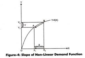
The graph made for this function shows a non-linear demand curve as depicted in Figure-4:
In Figure-4, at point A the value of X= XI and Y =Y1. With the increase in XI to X2, Y1 also increases to Y2. In such a case, we arrive at point B from point A.
Therefore, change in X would be represented as follows:
∆X = X2-X1
∆X = X2X1
Similarly, change in Y can be represented as follows:
∆Y=Y2– Y1
∆Y = Y2Y1
Therefore, the slope of the function can be expressed as follows:
Slope = ∆Y/∆X
Slope = Y2Y1/X2X1
Figure-4 shows a greater change in X and Y, which also results in large variations in the slopes of X and Y. However, for the function, Y = f(X), where ∆X approaches to zero. In such a situation, point B approaches to come back at point A. The technique to calculate the value of slope at which the fluctuation in independent and dependent variable is infinitely small is termed as derivative. Derivative can be calculated with the help of differentiation method.
The different functions of managerial decisions in which differentiation method is used are as follows:
i. Constant function
ii. Power function
iii. Sum or difference of two functions
iv. Product of two functions
v. Quotient function
vi. Function’s function
In the preceding functions, we would only explain the rules of differentiation that are the rules for determining derivatives of functions. In these functions, Y represents dependent variable, X as independent variable and a, b, and c are constants.
Let us understand the derivatives of these functions in detail.
Constant Function:
The derivative of the constant function is equal to zero. For example, in case the function is Y = f(X) = a, then
δY/δX = 0
This is because of the reason that the value of Y does not change with the value of X, which implies that the value of Y is constant. For example, in case of labor-capital ratio, capital is constant, and then the production function would be represented as follows:
Y = f(X) = 400
In such a condition, output (Y) remains same even if the labor (X) increases. This production function is represented as a horizontal line on a graph. The example of such production function is agricultural industry in India.
Power Function:
The derivative of the power function can be expressed as follows:
Y = f(X) = aXb
Where, a and b= constant
a= coefficient of X
b= power of X
The first derivative of the power function would be as follows:
δY/δX = baXb-1
Let us understand the derivative of power function with the help of the following examples:
i. If the production function is Y =4X3, then
δY/δX = 3*4* X3-1
δY/δX = 12X2
ii. If the production function is Y =3X2, then
δY/δX = 2*3*X2-1
δY/δX = 6X
Sum or Difference of Two Functions:
A dependent variable (Y) can be a function of a sum or difference of the two different functions that has same independent variable (X) or two other variables which are functions of X.
In case the functions of independent variable is a sum of the two different functions that has same independent variable, then the function can be expressed as follows:
Y = f (X) + g(X)
Where, f (X) and g(X) are the two different functions that represent different relationship between the dependent and independent variable. For the preceding function, the derivative can be described as follows:
δY/δX = δf (X)/δX + δg(X)/δX
In case, the production function is represented as follows:
Y = f (X) – g(X)
Then, the derivative can be expressed as follows:
δY/δX = δf(X)/δX + δg(X)/δX
Let us understand the application of the derivative of function of sum or difference of two different functions with the help of following examples:
(a) In case, the production function is Y = 5X + 2X3, then
δY/ δX = 5X1-1 + 2 * 3X3-1 = 5 + 6X2
(b) In case, the production function is Y = 5X2 – 2X4, then
δY/ δX = 2 * 5X2-1 – 4 * 2X4-1 = 10 – 8X3
Product of Two Functions:
The product of two different functions can be expressed as follows:
Y = f(X)*g(X)
The derivative of such functions can be represented as follows:
δY / δX = f (X) δg (x)/δx + g (X) δf (x)/δx
Therefore, the derivative of the product of two different functions can be expressed as the product of first function and the derivative of second function plus the product of second function and derivative of first function.
Let us understand the derivative of product functions of two different functions with the help of an example.
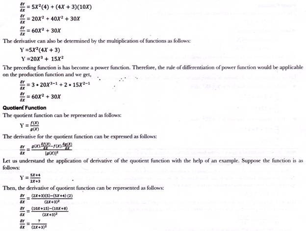
Suppose the production function is Y =5X2 (4X + 3), then the derivative of the production function can be calculated as follows:
Function’s Function:
There are certain functions in which one variable is a function of another variable. For example, the function of Y is Y = f (U) and the function of U = f(X). In case, we want to determine the derivative of Y with respect to X, then it would be equal to the product of derivative of Y with respect to U and derivative of U with respect to X, which is described as follows:
δY/ δX = δY/ δU * δU/δX
Let us understand the application of derivative of a function of function with the help of an example.
Suppose the two functions are as follows:
Y = U3 + 5U and U= 2X2
The derivative of Y with respect to U can be expressed as follows:
δY/ δU = 3U3-1 + 5
δY/ δU = 3U2 + 5
Putting the value of U in the preceding equation, we get
δY/ δU 3 (2X2)2 + 5
δY/ δU = 12X4 + 5
The derivative of U with respect to X can be expressed as follows:
δU/δX = 2 * 2X2-1
δU/ δX = 4X
The derivative of a function’s function can be represented a follows:
δY/ δX = (12X4 + 5)(4X)
δY/ δX = 48X5 + 20X
Partial Derivative:
There can be more than one independent variable in a function, such as demand function, production function, and cost function.
In such a case, the demand function can be expressed as follows:
Dx = f (Px, M, Py, Pc, T, A)
Where, Px = Price
M = Consumer’s income
Py = Price of substitute goods
Pc = Price of complementary goods
T = Consumer’s taste
A= Advertisement expenditure
Production function can be expressed as follows:
Q = f (L, K)
Where, L = labor
K = capital
The cost function can be expressed as follows:
C = f (K, r, L, w)
Where, L = labor
K = capital
r = rental rate
w = wage rate
For partial derivative, we have certain rules of differentiation. In partial differentiation, Y is assumed as the dependent variable and X and Z as independent variables.
The production function of partial differentiation is as follows:
Y = X3 +4XZ + 5Z2
The rules of partial derivation can be stated as under:
a. Permits change in one independent variable at a time
b. Adopts the same rule for differentiation as in case of one independent and one dependent variable
On the basis of preceding rules, we can calculate partial derivative.
When Z is constant, the derivative of Y with respect to X is equal to:
δY/δX = 3X3-1 + 4Z
δY/δX = 3X2 + 4Z
When X is constant, the derivative of Y with respect to Z is equal to:
δY/δX = 4X + 2*5Z2-1
δY/δX = 4X + 10Z
However, if the X and Z are in the form of a product as follows:
Y= aXbZc
Then, the derivative of Y with respect to X is as follows:
δY/δX = baXb-1Zc
Similarly, the derivative of Y with respect to Z would be as follows:
δY/δZ = aXbcZc-1
Optimization Techniques:
Optimization techniques are used to determine the value of independent variable that maximizes or minimizes the value of defendent variable. These techniques are useful for making various managerial decisions.
For example, generally, organizations strive to determine the level of output that would minimize the cost of production or maximize their profits. In this way, optimization techniques help in taking major decisions of an organization. Let us understand the techniques of optimization of various economic variables.
Maximizing Total Revenue:
Total Revenue (TR) can be determined by taking the product of price and quantity of a product that can be expressed a follows:
TR = P. Q.
Where, P= Price of product
Q = Quantity of product sold
For example, if a price function is as follows:
P = 250 – 2.5Q
Then, the total revenue would be:
TR = (250 – 2.5Q) Q
TR = 250Q – 2.5Q2
Now, we need to determine the value of Q at which the revenue is maximum. According to maximization rule of TR, the revenue produced from the sale of marginal unit of output should be zero.
Therefore, firstly, we need to determine the derivative of TR function as follows:
TR = 250Q – 2.5Q2
δTR/δQ = 250-5Q
By keeping the preceding equation of TR function to zero, we can determine the value of Q as follows:
250 – 5Q = 0
-5Q = -250
Q = 50
The maximum TR can be determined by putting the value of Qin the equation of TR function, which is as follows:
TR = 250*50 – 2.5(50)2
TR = 6, 250
The maximum value of TR can be checked by increasing or decreasing the value of Q by 1.
In case, the value of Q is 49, then the maximum value of TR would be as follows:
TR = 250(49) – 2.5(49)2
TR = 6,247.5
However, if the value of Q is 51, then the maximum value of TR would be as follows:
TR = 250(51) – 2.5(51)2
TR = 6,247.5
In both the cases, the value of TR is less than the value of TR when quantity sold is equal to 50. Therefore, the quantity sold should be equal to 50 for getting the maximum value of TR.
Optimizing Output and Minimizing Average Cost:
Optimum output can be defined as the output level at which the average cost of production for an organization is minimum. It helps in determining the most efficient size of an organization.
Determining the optimum size of an organization is helpful the future planning of the organization under certain conditions, which are as follows:
i. Helps in planning the set-up of a new production plant. An entrepreneur needs to know the optimum size of the production plant before establishing it. This is due to the concept of production theory, according to which there is a decrease in average cost to a certain output level. After reaching this level, the average cost starts increasing.
ii. Helps the organization to expand its scale of production. The size of the organization also enables the organization to plan and select appropriate marketing strategies.
iii. Helps small organizations to earn high profits and reduce per unit cost of production.
The formula used for the calculation of Average Cost (AC) is as follows:
AC = TC/Q
Let us assume that TC function of an organization is as follows:
TC = 200 + 30Q + 2Q2
By substituting the value of TC in the formula of AC, we get
AC = 200+30Q+2Q2/Q
AC = 200/Q + 30 + 2Q
According to the rule of minimization, the derivative of the function should be zero for minimizing the function. Therefore, we can determine the value of Q for minimizing Q with the help of the derivative of the AC function that can be calculated as follows:
δAC/δQ = -200/Q2 + 2
By equating the preceding equation with zero, we get
-200/Q2 + 2 = 0
Q2 + 200/2
Q = 10
When Q is equal to 10 units, the average cost is minimum. Therefore, 10 units is the optimum solution for the preceding problem.
Maximizing Profit:
Maximizing profit is the basic and most important goal of all organizations. Total profit (Π) refers to the difference between total revenue and total cost as expressed as follows:
Π = TR-TC
The profit would be maximum when the difference between the total revenue and total cost is maximum. Both TR and TC functions involve a common variable, which is output level (Q). In such a case, we need to determine the level of optimum output that maximizes profits.
This can be done in two ways, which are as follows:
i. Applying the rules of profit maximization
ii. Maximizing the profit function
Let us discuss these two ways in detail.
Rules of Profit Maximization:
The maximization of profit is possible under two conditions, namely, necessary’ or first- order condition and supplementary or second-order condition. Let us discuss the mathematical expression of these two conditions.
i. First-Order Condition:
Requires that MC should be equal to MR for the maximization of profit.
The mathematical representation of first-order condition is as follows:
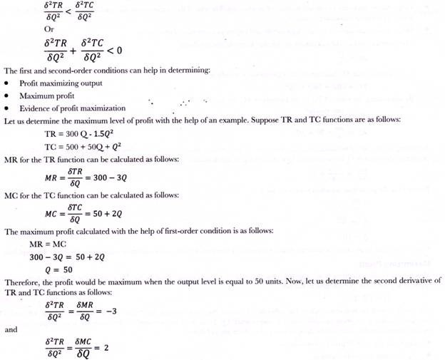
MR = MC
Or
δTR/δQ = δTC/δQ
δTR/δQ – δTC/δQ
Therefore, for maximizing profit, it is necessary that the derivative of TR and TC should be equal or their difference should be equal to zero.
ii. Second-Order Condition:
Requires that the difference of second derivative of TR and TC functions should be less than zero or their sum should be negative. Second derivative refers to the derivative of first derivative of a function.
Second-order condition can be mathematically represented as follows:
According to the second-order condition, profit would be maximum when the difference of second derivative of TR and TC function should be less than zero or their sum should be negative. In our case, the sum of derivative of MR and MC functions is equal to —1 (—3 + 2 = —1), which is less than zero. Therefore, it is satisfying both first and second-order conditions.
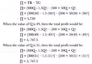
The value of output at which the profit is maximum (50 units) can be checked by increasing or decreasing the value of Q by 1.
Let us first determine the level of profit at output level of 50 units as follows:
In both the cases, the value of total profit is less than the value of total profit when the level of output is equal to 50. Therefore, the output should be equal to 50 for getting the maximum value of TR.
Profit Function Maximization:
In profit function maximization, we require to find out profit function and then maximize that function with reference to output.
The profit function can be determined with the help of TR and TC functions, which can be expressed as follows:
Π = (300Q – 1 .5Q2) – (500 + 50Q + Q2)
Π = 300Q – 1.5Q2 – 500 – 50Q – Q2
Π = -500 + 250Q – 2.5Q2
The derivative of the profit function would be a follows:
δΠ/δQ = 250-5Q
According to the rule of maximization, the derivative of profit function should be equal to zero. Therefore, keeping the derivative of profit function equal to zero, we can calculate the output level for profit maximization, as described in the following equation:
250-5Q = 0
Q = 50
Therefore, the profit would be maximum when the level of output is 50 units for the given TR and TC functions.
Multivariate Profit Maximization:
However, economists required to deal with more than one independent variable, such as labor and capital. Similarly, total revenue function has quantity sold and advertisement expenditure as independent variables.
In case of multi product fine, the profit function includes the profit of all products. Therefore, it is required to know the optimization of functions with more than one independent variable. Let us consider an example to understand the optimization of multivariate functions (having two independent variables).
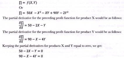
Suppose an organization produces two products, X and Y, then the profit function would be as follows:
The values of X and Y can be determined by multiplying the partial derivative of Y with 2 and then deducting the product from the partial derivative of X.
The value we get after the multiplication of 2 with the derivative of Y is as follows:
2(90 -X-4Y) = 0
180 – 2X – 8Y = 0
The value obtained from the difference of the preceding equation and the derivative of X would be:
(180 -2X- 8Y) – (50 – 2X – Y) = 0
130 – 7y = 0
Y = 19 (round off)
By putting the value of Y in the partial derivative of X we get:
50 -2X – 18.6 = 0
X = 16 (round off)
Therefore, to maximize the profit, the organization should produce 16 units of X and 19 units of Y.
In such a case, the total profit of the organization would be as follow:
Π = 50X – X2 – XY + 90Y – 2Y2
Π = 50(16) – (16)2 – 16*19+90(19) – 2 (19)2
Π = 1228
Linear Programming:
Linear programming refers to the mathematical technique used for solving optimization problems, such as maximization and minimization problems, of businesses. These optimization problems include variables that have linear relationships. In other words, linear programming provides the best solution for the allocation of resources and for the optimization problem under specific conditions. However, economic application of linear programming is very rare as it provides less information regarding the working of an economy.
Assumptions of Linear Programming:
There are certain assumptions made for solving the optimization problems with the help of linear programming.
These assumptions are as follows:
i. Linearity:
Assumes a linear relationship between input and output of production. It is not only an assumption, but also a condition for linear programming. According to the assumption of linearity, the factor of production provides equal returns in the short run. The linear relationship between input-output is represented by a linear equation. For example, a manufacturing company requires 25 men (W), 10 machines (M), and 0.6 tons of raw materials (R) for the production of one unit of output (O).
Therefore, the relationship between input-output can be represented as follows:
25W+ 10M + 0.6R= 10
However, this assumption has restricted the application of linear programming to linear input-output relationship only.
ii. Continuity:
Assumes that all variables are measurable only if they are having a numerical value. According to this assumption, only numerical values bring continuity in the measurement of variables.
iii. Independence and Additively:
Assumes that variables and their numerical values are not dependent on other variables. This implies that variables are .selected randomly within limits. Another assumption is related to the additive nature of variables to be added together. If variables cannot be added together, they have no meaning in linear programming.
iv. Proportionality:
Assumes that there is a proportional relationship among variables. The proportionality between the variables remains same while finding out the solution of the problem. This implies that the proportional relationship among variables is same at every level of output. For example, if a product requires 5 units of input to produce one unit of output, then the production of 10 units of output would require 50 units of input.
v. Constant Price:
Assumes that the prices of input and output remain constant, regardless of the quantity sold and purchased.
Application of Linear Programming Technique:
Linear programming technique help in business decision-making by finding out solution for various business problems, such as maximization of profit, minimization of cost, and expansion problems. Let us understand the application of linear programming in solving out these business problems.
Linear programming technique is most commonly used for solving out profit maximization problems. For example, an organization has two products, A and B that can be produced with the help of two inputs, P and Q. The requirement of total inputs per unit of time by the organization is equal to P = 800 units and Q = 1000 units. Profit produced per unit of A= Rs. 5 and B= Rs. 4.
The requirement of per unit input for the production of A and B are shown in Table-2:
The organization required to find out the combination of inputs for the maximum profit (Π). To solve the preceding problem with the help of linear programming technique, we need to form linear programming equations as described in the following steps:
1. Objective Function:
Refers to the first step of formulating the objective function for solving the problem. For Table-2, the objective function can be represented as follows:
Maximize π = 5A + 4B
In the preceding equation, A and B represent the quantity of output that would be multiplied by profit per unit to get the total profit. The linear programming technique is used to find out the values of A and B in the preceding equation.
2. Constraint Equations:
Help in determining the requirement of input to produce per unit of output and the total amount of profit available to the organization.
For example, for the present example, the constraint equation for P can be expressed as follows:
4A + 2B ≤ 800 P
The preceding equation implies that the total supply of input P is 800. Out of which 4 units of input P is used for the production of output A and 2 units of input P is used for the production of output B.
Similarly, we can find out the constraint equation for Q that can be expressed as follows:
2A + 5B ≤ 1000 Q
In case of Q the total supply is equal to 1000. Out of which 2 units of input Q is used for the production of output A and 5 units of input Q is used for the production of output B.
3. Non-Negativity Condition:
Refers to the condition required for getting the more realistic solution of maximization problem. It can be possible that the solution of linear programming contains a negative value, which is not possible in the real world. Therefore, to avoid such situation, non-negative approach is adopted.
In our example, the non-negativity condition can be expressed as follows:
A ≥ 0 and B ≥ 0
The complete linear programming equation can be expressed as follows:
Maximize π = 5A + 4B
Subjects to constraints.
i) 4A + 2B ≥800
ii) 2A + 5B ≥ 1000
Where, A, B ≥ 0
To solve the preceding linear programming equations, the graphical method is used discussed below.
Graphical Method:
Graphical method is considered and the problem of linear programming he simplest method for solving linear programming problems. In the graphical method, the problem of linear programming can be solved by transforming the unequal constraint equation into an equal constraint equation, which is expressed as follows:
4A + 2B = 800 and 2B + 5B = 1000
Now, we can plot the constraints on a graph by calculating the values of A and B with the help of terminal points.
The calculation of A and B values with the help of terminal points are shown as follows:
Suppose, for constraint equation 4A + 2B = 800, A = 0,
Then, B = 800/2
B = 400
In case, B = 0,
Then, A = 800/4
A = 200
Similarly, for constraint equation 2a + 5B = 1000, a = 0,
Then, B= 1000/5
B=200
In case, B = 0,
Then, A= 1000/2
A=500
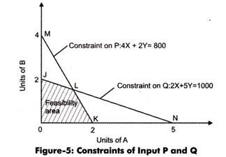
Let us plot the calculated equations of A and B on a graph, which is shown in Figure-5:
In Figure-5, OKM represents the feasibility area of P, while ONJ represents the feasibility area of Q. All the points that lie in the feasibility area are called feasible points. The shaded area, JLKO represents the points that satisfy all the conditions and assumptions of linear programming.
The points lie in area MLJ can only satisfy conditions of constraint P and LKN can only satisfy conditions of Q constraints only. JLKO is the only area that can satisfy the conditions of both P and Q constraints. In addition, it contains the solution of profit maximization problem.Now, we need to determine the point at which the combination of P and Q yields the maximum profit. This can be possible by plotting objective function on graph that would represent the iso-profit line for various output levels.
For this, we need to determine the slope of objective function as follows:
π = 5A + 4B
or B= [(π -5)/4] A
When Π = 0
B= (-5/4) A
Therefore, the slope of iso-profit line is equal to-5/4. This implies that the profit produced by one unit of B and 1.25 unit of A is same. With the help of slope of iso-profit, we can determine the various iso-profit lines and overlaid on the feasibility area for determining the point of maximum profit.
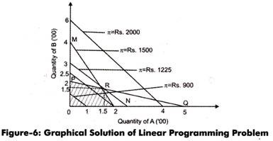
Iso-profit lines would be parallel because profit of A and B are constant, as shown in Figure-6:
In Figure-6, maximum profit of Rs. 2000 is not appropriate, as it does not feasible in the linear programming conditions. The iso- profits of Rs. 200 and Rs. 250 indicate the improper utilization of resources. Therefore, they would yield less profit. Only the iso-profit line of Rs. 1225 fetches the optimum utilization of resources; therefore, would yield maximum profit.
Thus, R is the point at which maximum profit can be generated, as shown in Table-3:
The combination of A and B for yielding maximum profit can be calculated as follows:
By constraint equation of P, we get
4A + 2 B = 800
A= (800-2B)/4
A= 200-(B/2)
Putting the value of A in the constraint equation of Q, we get
2A + 5B=1000
2[200 – (B/2)] + 5B = 1000
B = 150
Putting the value of B in equation (1), we get
A= 200-(150/2)
A= 200-75
A=125
Therefore, the maximum profit can be yielded when A= 125.and B = 150.
Cost minimization problem can also be solved with the help of linear programming technique. Let us understand it with the help of an example. Suppose a manufacturing organization requires 160 men (W’), 36 machines (M), and 48 tons of raw materials (R) for the production of product C and D.
The production conditions are given in Table-4:
The cost of production per product is Rs. 30,000 for D and Rs. 10,000 for C. The problem is to find out the output combination of products, C and D at the least cost.
The linear programming equation for the present problem would be as follows:
Minimize Cost = 10,000 C + 30,000 D
Subject to condition 10C + 40D ≥ 160
6C + 3D ≥36
4C + 8D ≥ 48
Where, C and D ≥ 0
The constraint equations with equality would be as follows:
10C + 40D= 160
6C + 3D = 36
4C + 8D = 48
Now, we can plot the constraint lines on a graph by calculating the values of C and D with the help of terminal points.
The calculation of the values of C and D with the help of terminal points is as follows:
Suppose for constraint equation of W, 10C + 40D = 160, C = 0
Then, D = 160/40
D = 4
In case, D = 0,
Then, C = 160/10
C = 16
Similarly, for constraint equation of M, 6C + 3D = 36, C = 0,
Then, D = 36/3
D = 13
In case, D = 0,
Then, C = 36/6
C = 4
For constraint equation of R, 4C + 8D = 48, C = 0,
Then, D = 48/8
D = 6
In case, D = 0,
Then, C = 48/4
C = 12
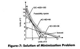
Let us plot the calculated equations of C and D on the graph as shown in Figure-7:
In Figure-7, MN line represents the line of labor constraint, JK and TR represents the line of constraints for other inputs. These lines are also termed as iso-cost. The optimum solution for the minimization problem lies in the feasibility space. The iso-cost line for optimum solution is IC.
The combination of output of C and D, at which the cost is minimum, is determined in Table-5:
In Table-5, the least cost is at point P of iso-cost line IJ. At point P, the production of C is 8 units while of D are 2 units.

