Kaldor’s Model of the Trade Cycle (With Diagram)

Read this article to learn about the Kaldor’s model of the trade cycle.

Kaldor’s theory of the trade cycle appeared in 1940 just four years after the publication of the General Theory in 1936.

It is a comparatively simple and very neat theory built directly on Keynes’ saving- investment analysis.

Although Keynes did devote a lot in the General Theory ‘Notes on the Trade Cycle’ and laid the basis for further discussion on the subject yet he did not develop a systematic theory of the trade cycle as such.

His theory of the determination of the level of income did not take into consideration the theory of the fluctuations of income, which received at his end a passing and scant attention.

It is important and interesting to note at the very outset that Kaidor’s theory of the trade cycle emerges essentially from the substitution of his particular non-linear saving and investment functions for the linear functions used by Keynes in his income model and from his intelligent tracing of the implications that follow from the quite different saving and investment relationships given by the nonlinear functions.

Kaldor in his trade cycle theory does not make use of the acceleration principle in a rigid form. In his model, investment is related directly to the level of income and inversely to the stock of capital. This approach, which is also associated with names like Kalecki and Goodwin, breaks the unrealistic, inflexible tying (or dependence) of investment to changes in output that is implied by the rigid acceleration principle (at the same time retaining the basic idea of the accelerator). Kaldor introduces an important variable that plays a major role in cyclical changes in saving and investment and this variable is the capital stock (K) in the economy.

Saving is a direct function of the capital stock, for any level of income, the greater the capital stock, the larger is the amount of saving. On the other hand, investment is an inverse function of the capital stock, for any given level of income, the greater the capital stock, the smaller is the amount of investment. In Kaidor’s cycle theory we try to trace out how the changes in the capital stock, that occur over time, alter the equilibrium situations.

In other words, and in short, instead of the investment function incorporating the strict acceleration principle I_t, + I_a+ w(Y,_t-1 – Y,_t-2), this approach gives us an investment function, which is like this: I_t = l_a + hY _t-1 –  jK₁; where K is the stock of capital at the beginning of the period t and where h and j are constants. The new equation simply means that if output or income (Y) increases while the capital stock (K) remains constant—investment will rise to increase the capital stock (other things being equal).

If, on the other hand, the capital stock increases while output or income remains constant—investment will fall as the desired stock of capital is (or has been) reached. The main difference between Hicks’ model of the trade cycle and Kaidor’s model is that the former uses the acceleration principle in its rigid form; while the latter uses it in a way as to avoid some of the shortcomings of the rigid acceleration principle. This is implied by the two equations given above on which investment at a time depends.

Kaidor’s model relying on Keynes’ model of income determination assumes that the process of change in the business activity is related to the difference between ex-ante saving and investment in the economy. If S > I, the savings are more than investments and there is a decline in consumer spending which through multiplier will bring a fall in income and business activity. If, on the other hand, I > S, then the income rises due to increased spending and higher investment. Thus, a discrepancy between ex-ante saving and investment induce a chain of reactions in the level of income till the equilibrium is restored.

Kaldor, thus, makes both S and I depend upon income (Y) and stock of capital (K), that is:

I = I (Y, K)

S = S (Y, K).

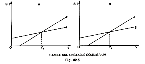
Both S and I are usually related to the level of income except in case of deep depression or extreme inflation, so that ∆I/∆Y and ∆S/∆Y are normally greater than zero. The behaviour of S and I in relation to the stock of capital, however, shows that saving is related positively with the accumulation of the stock of capital and vice-versa; while investment generally bears an inverse relationship with the stock of capital. The fluctuations (cycle) in the economic system can be traced to the movements of the variables like, I, S, Y and K. Now, if we suppose that S and I functions are linear (straight line curves), Kaldor, then, points out two possibilities as shown in the Fig 42.5.

In part A of the Figure, the equilibrium level of Y is Y_e—the only income level at which planned saving and planned investment are equal. With any given pair of linear S and I functions, there is a single equilibrium position and any disturbance that results in a shift in either function or both would tend to be followed by a movement to a new equilibrium position. But from the specific viewpoint of the business cycle, this model offers little help because it shows more stability than appears to be in the real world. In part B, there is again a single equilibrium position but it is unstable one.

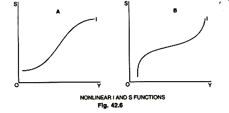
Any disturbance producing a movement above, Y_e means that I > S and that the income level may rise without limit, first to full employment and then beyond to hyper-inflation. Any disturbance leading to a movement below Y_e means that S > 1 and that the income level would collapse to zero output or income. Part B gives us greater instability than the real world shows. But as an explanation of the business cycle both the cases pointed out by Kaldor are found wanting, one for too much stability and the other for too little. Kaldor, therefore, concludes from this analysis that S and I functions cannot both be linear, at least not over the full arrange of income during the business cycle. Nonlinear S and I functions appear to conform more closely with the behaviour of saving and investment during the course of cycle as shown in Fig. 42.6.

In part A, the curve is almost flat for both relatively high and low income levels and the MPI is almost zero. The MPI is expected to reach zero at low income levels because there is already large excess capacity and rise in income at low point will not induce any investment spending.

Similarly, in case of high level of income, according to Kaldor, MPI will be small because of rising costs of business, construction, borrowing etc. which will discourage entrepreneurs to invest more. Thus, there is a range of income over which increases in income (∆Y) will be accompanied by small or zero increments to investment (∆Y) or ∆I/ ∆Y will be very small or zero over this range of Y.

Again in part B, at relatively high and low income levels, the MPS is relatively large compared to its magnitude at normal income levels. During recession when incomes fall to low levels, people cut saving to maintain their previous standards of living and at high income levels, people not only save a large amount but a larger proportion of their income, therefore, the MPS is high. This shifts the distribution of income in favour of profits and away from wages because the MPS of profit seekers is higher than the wage earners. This is reflected in a steep rise of the S function at high income levels.

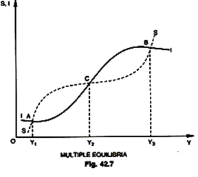
The Fig. 42.7 has been derived by combining the nonlinear I and S functions as shown below. This figure shows multiple equilibria, with both A and B as stable positions. At income levels below Y₁ or between Y₂ and Y₃ I > S, so the income level rises. At income levels between Y₁ and Y₂ or above Y₃, S > I, so the income level falls. C is an unstable position and, therefore, the income level Y₂ is not a possible equilibrium level.

If income is between Y₂ and Y₃, it will rise to Y₃, and if income is between Y₁ and Y₂, it will fall to Y₁. It appears that the economy can reach stability only at some high level of income Y₃, or at some low level of income Y₁. This, however, does not give us a complete model of business cycle, because a business cycle is made up of alternating expansions and contractions and this figure shows simply two possible positions of stable equilibrium.

According to Kaldor, “The key to the explanation of the trade cycle is to be found in the fact that each of these two positions is stable only in the short period—that as activity continues at either one of these levels, forces gradually accumulate which sooner or later will render that particular position unstable”.

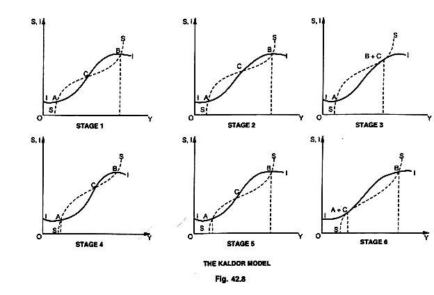
If indeed it can be shown that the stable equilibrium at A becomes unstable over time and forces a movement to B, we will have pushed ahead to a model of business cycle. This is apparent from the study of the models given in Fig. 42.8 by Kaldor.

The first stage of the Kaldor model given in Fig. 42.8 corresponds to the figure already given in the above paragraph. We start off in this with the assumption that the economy is in equilibrium position at B, which corresponds to a relatively high or above normal income, at which investment is also high but the higher the rate of investment, the more rapid is the increase in the size of the capital stock.

As the capital stock grows, it means MEC falls, which in turn, leads to a downward shift in the MEI curve, which is denoted here by a downward shift in the I curve (beyond point B). At the same time, the growth in the capital stock of the economy means a growth in the total wealth of the economy which in turn, will tend to push up the saving curve S (beyond point B in stage I of this Figure).

This means there is a rise in the average propensity to save in the economy induced by an increase in its wealth. As shown by stage 2 of the diagram, the downward movement of the I curve and the upward movement of S curve result in a gradual shift to the left in the position of B and a gradual shift to the right in the position of C so that B and C are brought closer to each other.

The critical point is reached when these gradual shifts of the I and 5 curves make the two curves tangential (tangent to each other at point B) and bring B and C together as is shown in stage 3 of the diagram. Now, at the position of B + C, S > I in both directions, and the equilibrium is unstable in a downward direction. The cyclical contraction, once started, reduces the income level until a new stable equilibrium is reached at the relatively low level that corresponds with A.

It may be noted that even A is a stable equilibrium only in the short-run. Over time, the S and I curves gradually shift, but now, with the system at a relatively low income level, the I curve shifts upward and the S curve shifts downward as shown by stage 4 in the diagram. If the level of investment corresponding to A is less than replacement requirements some inward shift in the I curve will occur sooner or later on account of replacement reasons alone.

Besides, as the time passes more and more investment opportunities develop, which means the MEC curve will rise and shift to the right pushing up the MEI curve which here would mean an upward shift in the I curve. At the same time, any decline in the capital stock or in the wealth of the economy that occurs during the period of low income will tend to lower the average propensity to save or push the 5 curve downward.

These shifts cause the position of A to move to the right and that of C to move to the left, thus, bringing A and C close together as is shown from stage 4 and stage 5 in diagrams. Again, the critical point is reached when these gradual shifts of the I and S curves makes the two curves tangential (tangent to each other at point A) and bring A and C together, as shown in stage 6 of the diagram.

The A + C position is unstable in an upward direction, since I > S on both sides of the position. The cyclical expansion, once started, raises the income level till a new stage of equilibrium is reached at the relatively high level that corresponds with B. The curves, thereafter, are likely to return gradually to the position shown in stage I of the diagram and another cycle begins.

The cyclical process, as described above by Kaldor is, thus, self-generating. The very movement to relatively high income levels brings into play forces, that after a period of time, produced a downward movement to relatively low income levels, and vice-versa. These forces, such as the changing size of the APS and the accumulation and de-cumulation of capital that occur over the cycle, are inherent in the economic process they are endogenous (within the system) forces in the full sense of the term.

One of the most important features of the Kaldor’s model of trade cycle is the impact or the importance of the distribution of income because the income of the society is distributed between different classes (Y – W + P i.e., wages plus profits), each of which has its own propensity to save, the equilibrium can be brought about only under a proper and appropriate distribution of income.

On the one hand, the relations of distribution determine the given level of social saving and, therefore, of investment, on the other hand, achievement of equilibrium (growth rate)’ requires a given level of investment and, therefore, of saving, which in turn, means corresponding distribution of income (provided the MPS of each class remains unchanged).

According to Kaldor, the introduction of the distribution mechanism (of income) into the model (with the proviso that Sp > 5V i.e., profit seekers savings are more than wage earners) makes the system more stable and more capable of automatically restoring equilibrium. Here we find Kaidor’s model differs materially from Harrod’s model. Kaldor believes that any change in I in relation to S—which in Harrod’s model will tend to produce cumulative processes of decline or growth in income and production—will set off (in Kaidor’s model) the mechanism of income redistribution, which adopts S to the new level of I.

Inflationary processes have an important part to play in this redistribution of income (necessitated by I > S or I < S). Kaldor assumes that when I > S, the rising investment and the general growth of demand under full employment will result in faster growth of prices than of wages, thereby, changing the distribution of income in favour of profit and reducing the share of the workers.

Because savings from profits are higher than the savings from wages (Sp > Sw), this will result in a growth of savings and the equality of S and I will be restored, if, on the other hand, investment and overall demand tends to decline, prices are likely to drop faster than wages, distribution will tend to change in favour of the workers, savings will decline, and the equality of S and I will be restored (though at low equilibrium level). In economic writings the equilibrium, thus, restored through the mechanism of income distribution is called ‘Kaldor Effect’.