In this article we will discuss about the demand function for commodities.
The quantity of a commodity to be demanded [purchased] by consumers depends mainly on its own price, cross price [prices of other commodities such as complementary and substitutes] and income. These factors are referred to as determinants.
Functional relationship between the quantity of commodity demanded and its determinants can be shown as follows:
Y = f (X1, X2, X3)
ADVERTISEMENTS:
Where,
Y = Quantity demanded [purchased]
X1 = Price of the commodity
X2 = Prices of other commodities [complementary/substitutes]
ADVERTISEMENTS:
X3 = Income
There will always be an inverse relationship between Y and X1; and a positive relationship between Y and X2. If it is a substitute and an inverse relationship if it is a complementary commodity.
In the case of normal commodities, there will be a positive relationship between Y and X3. In the case of inferior commodities, there will be an inverse relationship between Y and X3. Since four variables are considered in the demand function, the elasticities of Y with respect to X1, X2 and X3 have been explained.
Own Price Elasticity of Demand:
ADVERTISEMENTS:
Price elasticity of demand is a ratio of proportionate change in demand for a commodity to proportionate change in price as shown below;
eY.X1 = ∂Y/Y/∂X1/X1 = ∂ Y/Y. X1/∂X1 = ∂Y/∂ X1. X1/Y < 0 [The sign of eY.X1 will always be negative]
Cross Price Elasticity of Demand:
Cross Price elasticity of demand is a ratio of proportionate change in demand for a commodity to proportionate change in price of other commodities [which may either be complementary or substitute] as shown below.
eY.X2 = ∂ Y/Y/∂ X2/X2 = ∂ Y/Y. X2/∂ X2 = ∂ Y/∂ X2. X2/Y 0
If it is less than zero [i.e., negative], then the commodities under consideration will be complementary; If it is greater than zero [i.e., positive], then the commodities under consideration will be substitutes.
Income Elasticity of Demand:
Income elasticity of demand is a ratio of proportionate change in demand to proportionate change in income as shown below:
eY.X3 = ∂ Y/Y/∂ X3/X3 = ∂ Y/Y. X3/ ∂ X3 = ∂ Y/∂ X3. X3/Y 0
If it is greater than zero [positive], then the commodity under consideration will be normal; If it is less than zero (negative), then the commodity under consideration will be inferior. On the basis of the sign of the eY.X3, the nature of the commodity can be classified. In applied econometrics, the price, cross and income elasticities of demand for a commodity will be estimated from the linear and log-linear demand functions.
ADVERTISEMENTS:
Linear Demand Function:
The specification of linear demand function for a commodity will be as follows:
Y = b0 + b1X1 + b2X2 + b3X3+ error……………….. (33)
ADVERTISEMENTS:
Where
Y = Quantity demanded [purchased]
X1 = Prices of a commodity
X2 = Prices of other commodity [ complementary/substitutes]
ADVERTISEMENTS:
X3= Income
The partial derivative of Y with respect to X1 [marginal effect], keeping X2 and X3 constant, is
∂ Y/∂ X1 = b1 < 0
The partial derivative of Y with respect to X2, keeping X1 and X3 constant, is
If b2 > 0, then the commodity is a substitutes.
ADVERTISEMENTS:
If b2 < 0, then the commodities is a complementary.
The partial derivative of Y with respect to X3, keeping X1 and X3 constant, is
If b3 > 0; then commodity under consideration will be normal; If b3 < 0; then the commodity under consideration will be inferior.
The partial elasticity of Y with respect to X1, keeping X2 and X3 constant, is
eY.X1 = ∂ Y/∂X1 . X1/Y = b1. X1/Y < 0.
ADVERTISEMENTS:
The partial elasticity of Y with respect to X2, keeping X1 and X3 constant, is
eY.X2 = ∂ Y/∂X2 . X2/Y = b2. X2/Y 0.
The partial elasticity of Y with respect to X3, keeping X1 and X2 constant, is
eY.X3 = ∂ Y/ ∂X3. X3 /Y = b3. Y /X3 0.
In estimating the partial elasticities, one can use either total of X1, X2, X3 and Y or mean value of X1, X2, X3 and Y or individual values of X1i, X2i, X3i and Yi: In the empirical studies mean values will be considered to evaluate the price, cross price and income elasticities of demand.
Therefore these elasticities will be referred to as average own price, cross price and income elasticities. The values of b0 b1, b2 and b3 will be estimated by OLS method with specific assumptions relating to the distribution of random variable, independent variables and dependent variable.
ADVERTISEMENTS:
The reliability of the above estimates of b0, b1, b2 and b3 can as usual be assessed by taking the values of standard errors or Y values. If the standard errors are smaller than half of the regression coefficients of X1, X2 and X3 then the estimates are deemed to be reliable estimates i.e., X1, X2, X3 variables do have significant impact on the demand for the commodity.
If it is more than half of the regression coefficients, then the estimates of parameters are deemed to be unreliable estimates i.e., X1, X2 and X3 do not have significant impact on the demand for the commodity. Similarly, the value of ‘t’ test can be considered to assess the reliability of estimates of the parameters. If the values of ‘t’ are very high, then the estimates are considered to be statistically significant.
If they are smaller, then the estimates are considered to be statistically insignificant. Thus, on the basis of either standard errors or ‘t’ values, the reliability of estimates can be assessed. Similarly, the overall goodness of the linear equation fitted to time series data can be assessed by taking the values of both R2 and Adj R2.
If the value of these statistics are close to one, then the linear regression model [equation] fitted to the observations [data points] will be considered good. If the value of these statistics are close to zero, then the linear regression model fitted to the observations will be considered not good.
Thus, the values of R2 and Adj R2 provide us an idea about the extent of variation explained by the independent variables included in the model in total variation.
Log Linear Demand Function:
ADVERTISEMENTS:
If the linear regression model [Linear demand function] is found to be not suitable to the data points, then other forms of equations have to be attempted.
The most popular form of regression equation is log linear [double-log or Power or constant elasticity model] regression model or log-linear demand function, whose specification will be as follows:
log Y = log b0 + b1 log X1 + b2 log X2 + b3 log X3 + error ………………. (34)
The partial derivative of log Y with respect to log X1 , keeping other variables constant, is
∂ log Y/∂ log X1 = ∂ Y/Y/∂ X1/X1 = b1 which will be less than zero
Similarly, the partial derivative of log Y with respect to log X2, keeping other variables constant, is
∂ log Y / ∂ log X2 = ∂ Y / Y / ∂ X2/ X2 = ∂ Y / Y / ∂ X2/ X2 = b2 which will be less than or more than zero
The partial derivative of log Y with respect to log X3, keeping other variables constant, is
∂ log Y / ∂ log X3 = ∂ Y / Y / ∂ X3/ X3 = ∂ Y / Y.X3 / ∂ X3 = b3 which will be less than or more than zero
b1 is known as the price elasticity of demand. If its value is more than unity, then the proportionate change in demand will be higher than the proportionate change in price of the commodity showing elastic nature of the commodity to the changes in own prices, all else equal. If its value is less than unity then the proportionate change in demand will be smaller than the proportionate change in own price of the commodity, showing inelastic nature of the commodity to the changes in prices of the same commodity, all else equal.
If its value is unity then the proportionate change in demand will be equal to the proportionate change in price of the commodity. If the value of b2, the cross price elasticity of demand, is more than unity then the proportionate change in demand is higher than the proportionate change in prices of other commodities [which may be either complementary or substitutes]; If it’s value is less than unity then the proportionate change in demand will be less than the proportionate change in prices of other commodities.
If it is equal to unity then the proportionate change in demand will be equal to the proportionate change in prices of other commodities. If the sign of cross price elasticity of demand is negative then the commodity under consideration will be complementary. If the sign of cross price elasticity of demand is positive then the commodity under consideration will be a substitute.
Thus, on the basis of sign of the cross price elasticity of demand, the nature of commodity may be identified as complementary or substitute. If the value of b3, the income elasticity of demand, is more than unity then the proportionate change in demand will be higher then the proportionate change in income showing the elastic nature of the commodity. If its value is less than unity then the proportionate change in demand will be smaller than the proportionate change in income showing the relatively inelastic nature of the commodity.
If its value is equal to unity then the proportionate change in demand will be equal to the proportionate change in income showing the unitary elastic nature of commodity. If the sign of income elasticity of demand is positive then the commodity under consideration will be considered normal. If the sign of income elasticity of demand is negative then the commodity under consideration will be considered as inferior to other commodities.
Thus, on the basis of sign of the income elasticity of demand the commodities can be classified into normal and inferior. From the linear demand function, own price, cross price and income elasticities of demand will be evaluated at the mean values of X1, X2, X3 and Y.
Therefore, these elasticities are referred to as average price, cross price and income elasticities of demand. In the case of linear demand function the elasticities go on changing from point to point, if the elasticities are evaluated at different values of Y, X1, X2 and X3.
In case of double log demand function the elasticities will be constant. The ultimate choice of the model for demand function will be based on the value of adjusted R2, the statistical significance and sign of the regression coefficients. In brief the choice of the results of the demand function for the analysis, policy making and forecasting will be based on economic, statistical and econometric criteria.
Demand Function for the Commodities–Estimates of Economic Relationships:
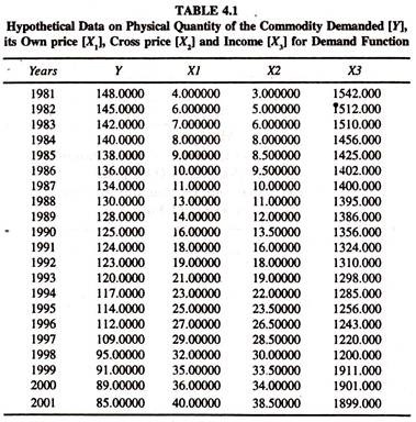
The following hypothetical data [Table 4.1] on physical quantity of the commodity demanded [Y], its own price [X1],cross price (prices of other commodities)[X2] and income [X3] are considered for estimating both the linear and log linear demand functions.
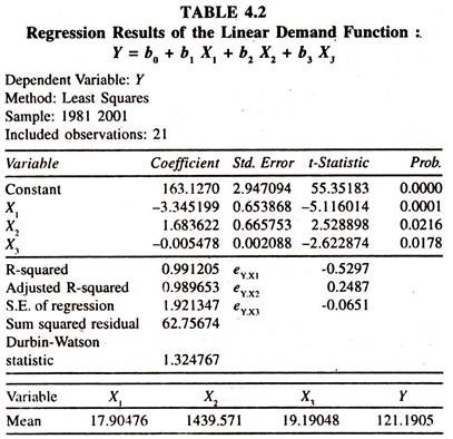
The results of the linear demand function [Table 4.2] show- that the regression coefficients of own price [X1], cross price [X2] and income [X3] are statistically significant. The own price, cross price and income elasticities of demand for the commodity [estimated at the mean values] are -0.529 [-3.345 (19.19/121.19)], 0.249 [1.6836 (17.90476/121.1905)] and – 0.0650 [-0.005478* (1439.57/121.1905) respectively.
The sign of cross elasticity of demand is negative showing that the commodities under consideration are complimentary. The sign of the income elasticity of demand is also negative showing that the commodity under consideration is not normal. The price elasticity of demand is negative and less than unity showing the inelastic nature of the commodity to the changes in prices of the same commodity, all else equal.
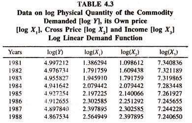
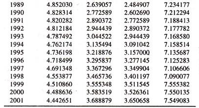
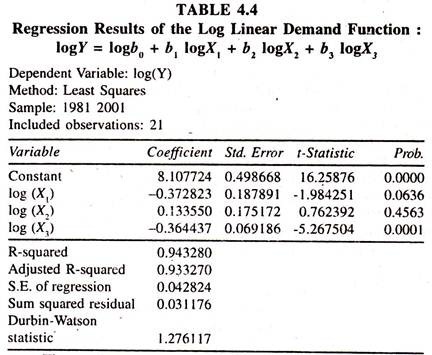
The regression results of the log linear demand function [Table 4.4] based on the data given in table 4.3 show that the regression coefficient of cross price [X2] is positive but not significant. The regression coefficient of income [X3] is significantly negative and the regression coefficient of own price [X1] is negative at low level of confidence.
It should be noted that the choice [linear or log linear form] of the results of the demand function depends on economic, statistical and econometric norms. In empirical studies, both the short run and long run demand functions [to estimate both the short run and long run price, cross and income elasticities of demand] for different commodities are estimated through the Nerlovian’s Partial Adjustment Mechanism using time services data.
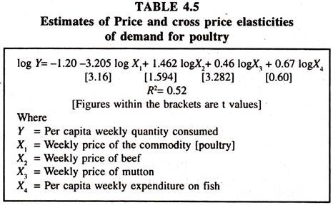
Time series family budget data will be used for estimating demand functions and demand elasticities. The budget data [concerned at a point of time] will however be not sufficient to estimate the price elasticities. In view of this, the price and cross price elasticities of demand for poultry in Mymensingh town, Bangladesh were estimated using panel data.The estimates of the study are given in Table 4.5.
The signs of the coefficients of the independent variables are positive showing that they are substitutes. Further the commodity beef was found to be close substitute as the elasticity value exceeded unity.
The price elasticity of the commodity, poultry is significantly negative evincing the fact that a one percent increase in the price of that commodity would reduce the demand for that commodity by more than three percent. It should be noted that the estimation of own price, cross price and income elasticities of demand for the commodities is not easy if the data points on the variables are not available in required form.
