Study Notes on the Employment Function | Econometrics

The below mentioned article provides a study note on the employment function.

Empirical Model for Employment Function from Cobb Douglas Production Function:

The employment [labour] intensity of economic growth can be understood by the size of output elasticity of employment. In other words the concept of output elasticity of employment in a particular sector of the economy helps in understanding the extent of labour absorption capacity of that sector in the Economy. From the prospective of the macro production function of the economy, the labour [demand for labour] with complementary factors of production produces national output or gross domestic product [income].

The demand function for labour can be derived either from the Cobb Douglas production function or Constant Elasticity of Substitution [CES] production function by solving the marginal product of labour equation for labour input variable. Demand for labour [Employment = E] can be derived from the demand for the commodities produced in industrial/agricultural sector. Wage payment is a reward for the labour for rendering services.

Under the conditions of perfect competition [profit maximization], every unit of labour is supposed to receive the reward [i.e., Wage = W] equal to the value of its marginal product (MP_E) i.e., MP_E = W. This represents the state of equilibrium and the absence of exploitation of the labour by the entrepreneurs, which is most ideal situation.

In empirical production function studies, the CES production function (SMAC: Solow, Minhas, Arrow and Chenery) is preferred to the Cobb-Douglas production function on the grounds that the elasticity of substitution [σ] between the inputs in the Cobb- Douglas would, all the time, be unity, though constant.

Further, it should be noted that the estimates of the parameters in the empirical demand function for labour [generated from the Cobb-Douglas production function] will all the time be unity as proved below:

O = A E^{β 1} K^{β 2} ……………(56)

Where

O = Output [Production]

K = Capital;

E = Employment

Marginal product of labour [MP_E] is derived from the above equation:

 

 

One of the necessary conditions for profit maximization [most desired ideal situation to explain that the labour will not be exploited] is

∂ O/∂ E = W [Where W is wage rate]

W = β₁ O/E ………………..(56a)

Equation 56(a) is solved for labour [E] input to derive the following demand function for labour

E = β₁ O W- …………………..(57)

Taking logarithms on both sides of the equation [57] we obtain

logE = log β₁ + log O – logW …………………(58)

Thus the numerical values of the regression coefficients of output [output (O) elasticity of employment] and Wage rate [wage rate (W) elasticity of employment] are restricted to unity i.e. [∂ logE/∂ log O = 1 and

[∂ logE/∂ log W = -1]

The choice of CES production function for generating empirical demand function for labour input seems to be appropriate only if the estimates of parameters of the equation are significantly different from unity. The demand function for labour can be derived from the CES production function under marginal productivity condition to know the labour absorption capacity.

Empirical Model for Employment Function from CES Production Function:

The following constant elasticity of substitution [CES] production function is used to derive employment function by equating marginal product of labour to wage rate.

Specification of the C E S [SMAC] production Function

O = A [δ K^-p+ (1-δ) E^-p]^–η/p (59)

Where

O = Production [Output]

K = Capital

E = Employment (Labour)

A = Efficiency parameter; A > 0

η = Returns to Scale parameter; η > 0

δ = Distribution parameter ; 0 < δ <1

ρ = Extent of substitution [between K and E] parameter, P > -1, and related to the elasticity of substitution:

σ = 1/1+ ρ

Marginal product of labour [MP_E] from Equation 59 is derived as follows:

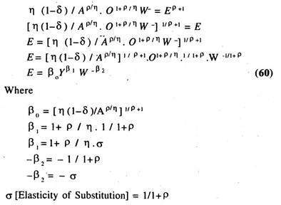
∂ O/ ∂ E= η (1-δ) A^p/η. O ^{(1+ ρ)/η} /E^{ρ +1}

An ideal situation [i.e. in which labour is not exploited] will be attained by equating marginal product of labour to wage rate

 

 

Equation 59(a) is solved for labour [E] input to derive the following demand function for employment

 

 

 

 

 

 

 

 

 

 

 

Taking logarithms on both sides of equation [60] we obtain

log E = log β_o+ β₁ log O – β₂ log W ……………(61)

log [Employment] = log β_o+ β₁ log [Production] – β₂ log [wage rate]

[1] The partial derivative of log E with respect to log O [output], keeping log W as constant, is

[∂ log E / ∂ log O = β₁ > 0] the constant output elasticity of employment.

[2] The partial derivative of log E with respect to log W [wage rate] keeping log O constant is

[∂ log E/∂ log W = -β₂ < 0] the constant wage rate elasticity of employment

Short Run and Long Run Employment Functions:

With a view to estimate both the short-run and long-run employment elasticities the following long run demand function for employment function will be hypothesized:

 

 

 

Where

E*_t = Desired level of employment in year t

O_t = Total Production in year t

W_t = Wage rate in year t

Since the desired level of employment is not directly observable, the following equation, which specifies the process of adjustment of actual to desired level of employment, will be introduced:

 

 

Where

E_t* = Desired level of employment (which is not directly apparent).

log E_t – log E_t-1 = Actual change in employment

log E_t*- log E_t-1, = Desired change in employment

λ = Speed of adjustment co-efficient

O < λ ≤ 1

if λ = 0, then E_t = E_t-1; If λ < 1 then actual change in employment will be lower than the desired change in employment (E_t/E_t-1 < E₁*/E_t-1); If λ = 1 then actual change in employment will be equivalent to desired change in employment. The equation (63) states that a constant percentage of the discrepancy between the actual and desired level of change in employment can be eliminated within a single period.

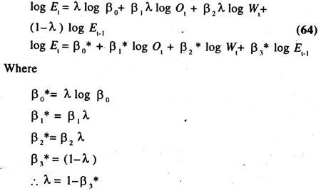
Substituting log E_t* (62) into (63) and re-arranging, we obtain the equation (64) known as the short run employment function. This equation states that the demand for labour in current year [t] depends on the production, wage rate in current year [t] and demand for labour in previous year [t-1]

 

 

 

 

 

 

 

 

 

 

∂ log E_t/∂ log O_t = β₁*> 0; The short run output elasticity of employment.

∂ log E_t/∂ log W_t= β₂*< 0; The short run wage rate elasticity of employment.

The long run elasticities will be estimated by deflating the short run elasticities with λ as shown below.

β₁^*/λ = Long run output elasticity of employment

β₂^*/λ = Long run wage rate elasticity of employment.

The long run employment function will also be estimated by deflating the short run employment function by λ and omitting log E_t-1 as shown below:

 

 

From the long run employment function, the long run output and wage rate elasticities will be estimated.

Employment Function by Solving Marginal Product of Labour for Labour Input:

The following form of employment function [regression model] will be generated from the CES production function [by solving the marginal product of labour for labour input variable].

Specification of the C E S [SMAC] Production Function

O= A [δ K ^-ρ + (1-δ) E^-ρ] ^–η/p ……………..(66)

Where

O = Output [Real Gross Domestic Product (GDP) at factor cost [Income]

K = Capital

E = Employment (Labour)

A = Efficiency parameter; A > 0

η = Returns to Scale parameter; η > 0

δ = Distribution parameter; 0 < δ < 1

ρ = Extent of substitution [between K and E] parameter, ρ > -1, and related to the elasticity of substitution;

σ = 1/1+ρ

The partial derivative of labour [Marginal product of labour [MP_E] ] from the above Equation is derived as follows:

 

 

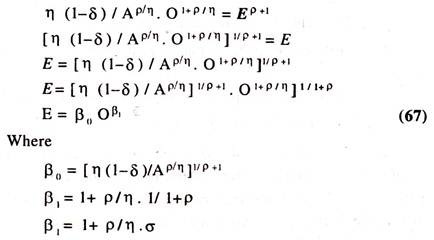
and the expression [MP_E ] η (1 – δ)/A^p/η. O ^{(1+P) / η}/E^ρ+1 solved for labour [E] input variable to derive the following empirical demand function for employment

 

 

 

 

 

 

 

 

 

σ [Elasticity of Substitution] = 1/1 + ρ

Taking logarithms on both sides of equation we obtain the following employment function:

log E_t = log β_o+ β₁ log O_t …………………(68)

This explains that the expansion of employment opportunities in any sector/economy, all else equal, mainly depends on the expansion of output [Production] in the respective industry/economy.

Empirical Model to Scan the differential Output Elasticity of Employment:

The degree of differential output elasticity of employment during post economic reform period [Policy Variable] can be scanned by fitting the following form of regression model with an interaction variable [D*log O_t]

log E_t = log β₀ + β₁ logO_t + β₂D + β₃ (D *log O_t) + error …………..(69)

Where

E_t = Employment

O_t = Output or Income [Real Gross Domestic Product (GDP) at factor cost]

Β₀= Intercept during pre reform period [D = 0]

β₂ = Differentia] intercept during post reform period [D = 1]

β₁ = Magnitude of output elasticity of employment during pre economic reform period (D = 0); β₁ > 0

β₃ = Magnitude of differential output elasticity of employment [shift parameter] during post economic reform period (D = 1); β₃more than or less than zero evinces the difference between the Magnitude of output elasticity of employment, during post economic reform period and Magnitude of output elasticity of employment during pre economic reform period

(β₁ ± β₃) = Magnitude of output elasticity of employment during post economic reform period (D = 1)

If the regression coefficient of dummy variable [D], β₂ is significantly positive then the average employment would go up during post economic reform period [D = 1] ;If it is significantly negative, then the average employment would go down.

If it is statistically insignificant then the average employment remains stable, β₁ = regression coefficient of O, constant employment elasticity [ β₁> 0] during pre economic reform period when D = 0, β₃= differential coefficient of employment elasticity, [β₃ more than or less than 0] that allows a shift [an upward/a downward] in the magnitude of output elasticity of employment during post economic reform period when D = 1.

As the interaction variable [D*log O_t] enters the equation in dichotomous form [i.e., D = 0 in pre economic reform period and D = 1 in post economic reform period] the derivative of logE_t with respect to [D*log O_t] does not exist. Instead, the coefficient of [D*log O_t], subject to statistical significance, measures the discontinuous effect of the presence of an attribute [D = 1] represented by an interaction variable on employment.

The variable [D*log O_t], which is known an interaction variable, is introduced in the above model to capture the interaction effect of economic reforms and output on employment.

The interaction variable takes a value equal to log O_t during post economic reform period [when D = 1] and 0 during pre economic reform period [when D = 0]; If [β₁^* ± β ₃^*] more than or less than β₁* then there will be an upward or a downward shift in the magnitude of output elasticity of employment during post economic reform period;

If [β₁* ± β₃**] = β₁*, then there will be a homogeneity in the magnitude of differential output elasticity of employment i.e., magnitude of output elasticity of employment remains the same in the pre and post economic reform periods [Where * and ** denote statistically significant and insignificant respectively]

Employment Function [Demand Function for Labour]—Estimates of Economic Relationships:

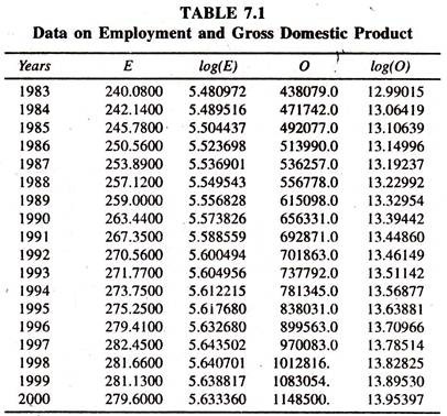
The data [Table 7.1] on Employment in organized Public and Private sectors [E] Output [Gross domestic Product [GDP] at factor cost at 1993-94 prices are considered to estimate employment function.

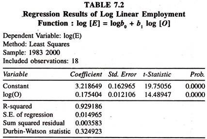
The regression results of the log linear employment function [Table 7.2] show that the regression coefficient of log Output [income],which is employment elasticity, is positively significant showing that a one percent increase in income leads to increase the employment by 0.18 percent per annum, all else equal.

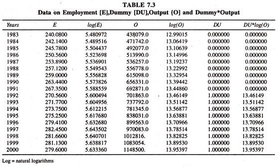
The data given in table 7.3 are used to scan the presence of shift in the degree of employment elasticity.

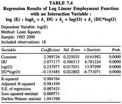
The regression results of the log linear demand function for labour with an interaction variable [Table 7.4] show that the employment elasticity during the pre economic reform period is positive but less than the elasticity of employment during post economic reform period as the differential coefficient during post economic reform period is negatively significant.

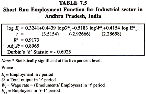
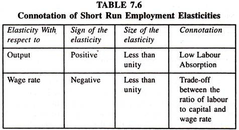
The Empirical Results of the short-run and long-run employment functions based on time series data [Tables – 7.5, 7.6 and 7.7] show that all the regression coefficients are statistically significant with expected signs. The short-run elasticity of employment with respect to production is 0.44 suggesting that an increase in production by one per cent leads to increase the employment by 0.44 per cent in the industrial sector of Andhra Pradesh.

This is in line with Okun’s Law according to which the elasticity of employment with respect to production will be less than unity. The regression co­efficient of wage rate, the elasticity of employment with respect to wage rate, is negative and less than unity suggesting that an increase in wage rate (labour cost) by one per cent leads reduce the employment by 0.52 per cent per annum in the Industrial Sector of Andhra Pradesh.

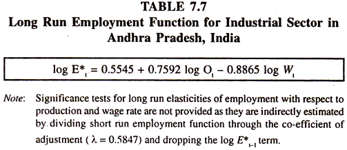
If the rate of growth of production of industrial sector in Andhra Pradesh is maintained, the cumulative effect of short run elasticity of employment with respect to production over a long period increases the employment by 0.76 per cent (Table 7.7) provided the wage rate remains constant.

The cumulative effect of short run elasticity of employment with respect to wage rate reduces employment by 0.89 per cent provided the production remains constant. The long run elasticities [Table 7.7] are substantially greater than the corresponding short run elasticities given in Table-7.5.

The co-efficient of employment lagged by one year is statistically significant showing the existence of significant lag in the adjustment of actual labour absorption to its desired level. The value of co-efficient of adjustment is λ = 1 — 0.4153 = 0.5847 implying that about 58 per cent of discrepancy between the desired level of employment and actual employment can be eliminated in a year in the industrial sector of Andhra Pradesh, India.