Modern Welfare Economics (With Diagram)

We have examined the maximisation problem of modern welfare economics within the framework of the simple 2 x 2 x 2 static model.

We turn now to the examination of its assumptions, to see which are simplifying, in the sense that they can be relaxed without essentially affecting the model, and which are restrictive, in the sense that if they do not hold the model collapses.

1. Extension to Many Factors, Products and Consumers:

The model can be extended to any number of resources, commodities and con­sumers.

2. Corner Solutions:

We have implicitly assumed that the two sets of isoquants provide a smooth locus of ‘internal’ tangencies, that is, the contract curve of production was assumed to lie inside the Edge-worth box. This assumption is not particularly harmful to the model. To cover cases where the tangency of the isoquants occurs outside the Edge-worth box of production (in which case the solution will be on the axes of the box, that is, there will be a ‘corner solution’) we must state the condition of equilibrium of production in the form of an inequality rather than an equality of the MRTS_L,K. In particular the condition.

MRTS^x_L,_K = MRTS^y_L,_K

must be replaced by the condition

(MRTS^x_L,_K) < (MRTS^y_L,_K)

or

{slope of the X isoquants} < (slope of the y isoquants)

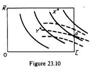
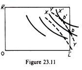
To understand this consider the figures 23.10 and 23.11.

Point a in figure 23.10 represents a ‘corner solution’. At a the slope of the X isoquant is smaller than the slope of the Y isoquant, so that a shows the maximum output of X (i.e. X*) given the output of Y (Y* in figure 23.10).

Point b in figure 23.11 is not an equilibrium solution, because it does not show the maximum of X, given Y. Actually, given Y, the maximum quantity of X is at point b’. (Apparently X’ > X). Note that at b the slope of the X isoquant is larger than the slope of the Y isoquant, so that the ‘inequality’ equilibrium condition is not satisfied.

In summary, for a corner solution to occur the Y isoquant must cut (on the axis of the Edge-worth box) the X isoquant from below.

3. Existence of Community Indifference Curves in Output Space:

The bliss point, where the social welfare function was maximized, was defined in utility space, that is, on the graph on whose axes we measure the utilities of the two consumers (in ordinal indexes), while the utility-maximising position of an individual consumer is determined in output space (i.e. on a graph on whose axes we measure the quantities of the two commodities).

The social welfare contours are not social or community indifference curves (equivalent to a single individual’s indifference curves). For a single individual, a given X Y combination (in output space) belongs to a unique indifference curve and has a unique slope (MRS^A_x,y).

However, if the particu­lar X Y combination is distributed between two consumers, a community indifference curve passing through XY (in output space) would not have a unique slope, because this slope would be sensitive to the way that the product mix XY is distributed among the two individuals. Recall that a particular product-mix can be distributed optimally among A and B in an infinite number of ways, along the contract curve of the Edge-worth box of exchange corresponding to this product mix.

Each distribution (of the given product-mix) has a different (equalized) MRS for the two individuals, because it corresponds to a different utility combination. These utility combinations, corresponding to the different distributions, form the utility possibility frontier for the particular commodity-mix.

Accordingly, the community MRS at a given point in commodity space (i.e. the slope of a community indifference curve) will vary with movements along the corresponding utility possibility frontier (i.e. with the distribu­tion of the XY combination between A and B).

In summary, we can say that a point in output space maps to a curve in utility space; and a point in utility space maps into a curve in output space. Not just one, but many possible XY combinations can yield a specified U_AU_B mix. It is this reciprocal point-line phenomenon that lies at the heart of Samuelson’s proof of the non-existence of community indifference curves.

The community MRS for a given fixed Y and X combination depends on how X and Y are distributed among A and B, i.e. on which U_AU_B point on the Edge-worth contract curve of exchange is chosen. Hence the slope of a community indifference curve for a given XY mix is not uniquely determined.

However, if one can decide which is the most desirable U_AU_B combination for a given ‘basket’ of X and Y, then the equalised MRS of the two individuals at this utility combination can be considered as the unique MRS of the community as a whole, so that the community indifference curve at the X Y point will have a unique slope.

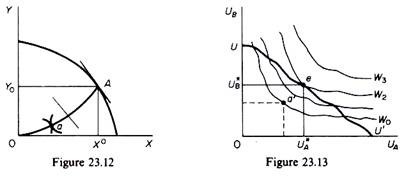
Based on this, Samuelson proved that one can derive community indifference curves by continuous redistribution of ‘incomes’ until the welfare function (axiomatically assumed to exist) is maximised in utility space. To illustrate this assume an initial distribution (point a in figure 23.12) which yields a total welfare of W₀ (point a’ in figure 23.13). With continuous redistribution the community can reach point e on W₂ where the social welfare is maximised for the particular Y₀ X₀ output mix. (We saw that e is mapped into a single point in output space.)

If we repeat this process for all output combinations, we can derive a set of social indifference curves in the output space.

Note the two basic assumptions of Samuelson’s proof of ‘existence’ of social indifference curves:

(a) A social welfare function exists;

(b) continuous redistribution of incomes’ is possible.

In summary, the maximisation of social welfare procedure can be used to ‘estab­lish’ the existence of community indifference curves in output space. These curves are called ‘community indifference curves corrected for income distribution’. They are widely used in international trade theory and in other fields of economics. Bator (op. cit.) argues that these community indifference curves reveal the society’s ranking of preferences, as reflected in a social welfare function which is defined by a government elected by political consensus.

Bator believes that the rankings of the society, based on these community indifference curves is more objective than that of any ‘arbitrary ethic standard’, adopted subjectively by policy-makers. We think that this argument is ‘circular’, since the community indifference curves (in output space) are derived from a social welfare function which is assumed to exist axiomatically, and which incorporates the subjective value judgements of those who supposedly have defined it. The point is that, given the subjective nature of the welfare function, the commun­ity indifference curves will also reflect subjective valuations.

4. Elastic Supply of Factors:

The 2 x 2 x 2 model assumed given quantities of factors. This assumption can be relaxed. The supply of factors can be expressed as a function of all the prices in the system. This allows for some elasticity in the supply of factors. The analytical effect is to make the PPC a function of the factors of production. This approach has been adopted in the generalized H x M x N model.

5. Joint and Intermediate Products:

It was assumed in the 2 x 2 x 2 model that all products were final products, and joint products were ignored. The model can easily be extended to take into account joint production of some goods, as well as the fact that some products are partly bought by final consumers and partly by other firms which use them in their produc­tion as inputs. Analytically this is done by introducing the relevant products as inputs in the production functions of the firms.

6. Decreasing returns to scale:

We have assumed constant returns to scale. If this assumption is relaxed and instead it is assumed that there are decreasing returns to scale, some problems do arise. In the case of decreasing returns the total value of output will exceed the total payments to the factors of production: product is not ‘exhausted’ by factor payments. This creates ambiguity about how to treat the imbalance between total value of output and total payments to factor owners in a general equilibrium framework.

Traditionally, decreasing returns to scale (increasing costs) are attributed to man­agerial diseconomies arising from the ‘entrepreneurial factor’ which is scarce even in the long run. Entrepreneurship, in this approach, defines the size of the firm (which is indeterminate in perfect competition with constant or increasing returns to scale), but is not treated explicitly as an input.

In any case no serious problems arise by assuming decreasing returns to scale. The required convexity of the production possibility curve is preserved, although the mathematical treatment of the problem becomes more tedious with the introduction of non-linearities.

7. Externalities divergence between private and social costs and benefits:

In our welfare-maximisation analysis we have assumed that there is no direct interaction among producers (independence of production functions), among hous­eholds (independence of utilities) and between producers and households.

Furthermore, in asserting the Pareto-optimal properties of perfect competition we have implicitly assumed that all benefits and costs of producers and consumers are reflected in market prices, and that there is no divergence between private and social costs and benefits. However, there are many situations in which the effects of an individual’s action is not fully reflected in market prices, and there is a difference between private and social costs and benefits.

When the action of an economic decision-maker creates benefits for others, for which he is not paid, there occurs an external economy for the others (and the economy as a whole). When the action of an individual agent creates costs for others for which he does not pay, there occurs an external diseconomy for the others (and the society as a whole).

The term externalities refers to both external economies and diseconomies. If externalities exist, the model breaks down for two reasons: first, the Pareto- optimality conditions are violated; second, the constants embedded in the system lose their significance as ‘prices’, because they do not reflect all the costs and benefits of an action to the society as a whole.

In other words, externalities create a diver­gence between private and social costs and benefits. Because externalities are not reflected in market prices, these prices provide misleading information (signals) for an optimal allocation of resources. We will examine separately the externalities in production and the externalities in consumption.

A. Externalities in Production:

(a) Divergence between Private and Social Costs:

We will illustrate this case with an example. Assume that commodity X is alcohol, which for simplicity we assume is manufactured in a perfectly competitive market. Each firm is in equilibrium when

MC_X = P_x

where MC_X is the cost of the individual firm, or the private cost. This does not include the cost of pollution of the environment that the firm creates, nor the costs of accidents and deaths caused by drunken consumers. These are external costs to the firm. Suppose that the Health Department obtains an estimate of these costs. The marginal social cost (MSC) is the sum of the private cost (MC_X) and the marginal external cost (MEC), that is

MSC_X = MC_X + MEC

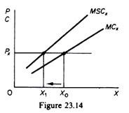
Obviously we have a divergence of private and social cost of alcohol. Since MC_X = P_x, it follows that P_x < MSC_X, which implies that the allocation of resources to the production of alcohol is not socially optimal; since the firm does not pay the full cost the production of alcohol in the economy is excessive. If the firm were made to pay the full social costs it would produce a smaller amount of alcohol, defined by the point where

P_x = MSC_x

This is shown in figure 23.14. The marginal social cost curve lies above the private marginal cost curve, given MSC_X > MC_X. The vertical difference between these two curves is the marginal external costs incurred in the production and consumption of alcohol. If the firm does not pay the external costs, its profit-maximising output is X₀. However, if the government required the firm to pay the external costs the firm would reduce its output to X₁.

In summary, when the private cost is smaller than the social cost, adherence to the rule MC_X = P_x leads to overproduction of X. By an analogous argument it can be shown that if MC_X > MSC_X, the level of production of X will be less than the socially optimum. Divergence between private and social costs (and benefits) results to misallocation of resources in a perfectly competitive system.

(b) Divergence between Price and Social Benefit:

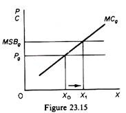
Even if the price is equal to the MSC there is no guarantee that social welfare is maximised, because price may be different than the social benefit. For example assume that an environmentalist uses unleaded petrol for running his car, paying P_g = MC_g. By using unleaded gasoline the environmentalist keeps the air cleaner, thus creating a benefit to others who breathe in a less polluted atmosphere.

Since they do not pay for this benefit we have an externality for the society as a whole. If we add the value of this benefit to the price we obtain the marginal social benefit (MSB). Apparently P_g < MSB_g, and since the firm produces where P_g = MC_g, it follows that the production of gasoline is less than the socially optimal quantity. If the govern­ment added the external benefit on the price of petrol, the consumers would pay the full MSB_g, and each firm would increase its production. This is shown in figure 23.15.

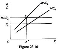
The MSB curve is above the P_g curve at all levels of output. If consumers pay the full MSB_g, the firm would increase its output by the amount X₀X_1. If we take into account any external costs of lead-free petrol the marginal cost curve would shift to the left (figure 23.16) and equilibrium would be reached at point e, where

MSC_g = MSB_g

From the above discussion we may conclude that when externalities exist, the condition for a socially optimal production is the equality of the MSC and the MSB. In a multi-product economy the condition for optimal resource allocation is

MSB_X / MSC_X = MSB_y / MSC_y = … = MSB_M / MSC_M = 1

(c) External Economies in Production:

We said that the presence of externalities in production invalidates the conditions required for social welfare maximisation. The question is how important are external­ities in the real world.

Some examples may illustrate the extent of the problem:

(i) A new highway reduces the transport cost of individual firms. Since they do not pay for the construction of the highway the MSC is higher than the private marginal cost.

(ii) The expansion of an industry (for example the motorcar industry) creates additional demand for the industries that supply it with raw materials, intermediate products and machinery. This increase in demand in the other industries may allow them to reap economies of large-scale production and lower the price of their prod­uct. This is an external economy to all the buyers of the product of these industries.

(iii) A new training programme of corporation A increases the supply of skilled labour for other firms in the industry. Since the latter do not pay the training costs there is an external economy for them.

(iv) If an apple producer grows more apple trees the production of a honey producer in the vicinity of the orchard will increase, because his bees have access to a larger number of apple trees. This is an external economy to the honey producer.

(v) If a honey producer expands his beehives the production of oranges of the owner of a near-by orange grove will increase, since bees help pollinate oranges. This is an external economy for the orange producer.

(vi) If a firm adopts a production method which reduces the pollution of a lake where it disposes its wastes the fish catch will increase. This is an external economy for fishermen in that lake.

(vii) Government-financed research creates external economies for all the firms which benefit from such research.

(d) External Diseconomies in Production:

(i) Pollution of lakes, rivers and the sea by firms reduces the fish population and hence creates an external diseconomy for the fishing industry. Pollution of this sort creates also health hazards, and therefore a diseconomy for all consumers in adjoin­ing areas.

(ii) Pollution of the air from the smoke of factories or fumes of cars and airplanes has similar diseconomies.

(iii) Establishment of a new industry in an area increases the wage rates to all firms in that area.

(iv) Creation of new shopping centres increases traffic in the neighbourhood, causing a diseconomy to the inhabitants of that area.

The above examples show that externalities in production are very important in the real world.

B. Externalities in consumption:

We have assumed that the utility level (satisfaction) of one consumer is indepen­dent of the consumption pattern of the other. This is a far cry from reality. Changes in fashion create strong imitation patterns (bandwagon effects). The desire ‘to keep up with the Joneses’ creates conspicuous consumption patterns (Veblen effect) which decrease the utility of at least some consumers. Snob behaviour is a widespread phenomenon in western societies.

The utility of snobs is greatly affected by the purchases of other people. A smoker decreases the utility of non-smokers in a restaurant or a theatre. The change of cars every year by some consumers decreases the utility of those who cannot afford such change. If one keeps one’s car in good condition, the safety of others, and hence their utility, is increased.

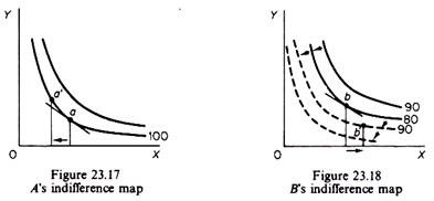
If externalities in consumption are present the equalization of the marginal rate of substitution of commodities among consumers does not lead to Pareto optimality and maximisation of social welfare. Consider figures 23.17 and 23.18, which show the indifference maps of consumers A and B. Assume that initially the two consumers are at points a and b where MRS^A_x,_y = MRS^B_x,y i.e. the condition of Pareto optimality in exchange holds if there are no externalities in consumption. Consumer A has a utility of 100 while consumer B has a utility of 80. (Utility indexes are used.)

Suppose that A is not affected by B’s consumption, but B’s utility is reduced by A’s consumption of commodity X (for example tobacco), but not of Y (for example alcohol). Under these conditions a redistribution of the same total output of X and Y between the two consumers can increase social welfare.

Assume that redistribution is such as to decrease the consumption of X by consumer A. This shifts the utility map of B downwards, showing the increase in the utility of B arising from the reduction in the consumption of X by consumer A. Redistribution is such that consumer A moves to point a’ and consumer B moves to b’. The total welfare has increased, despite the fact that at the new equilibrium the MRS_{X, y} is not the same for the two consumers.

In the new situation consumer A is on the same indifference curve, while B has moved to a higher indifference curve (point b’ lies on the shifted indifference curve with utility 90). We conclude that, when externalities in consump­tion exist, adherence to the equalisation of the MRS of the two consumers does not ensure Pareto optimality.

8. Kicked Isoquants:

We have assumed that the isoquants are continuous and smooth, without kinks. Such smooth curvatures are mathematically convenient, because calculus can be applied in the solution of the problem of welfare maximisation. Kinked isoquants cause indeterminacy in marginal rates of substitution, that is, lead to a breakdown of calculus techniques.

However, kinked isoquants can be handled with the linear pro­gramming techniques. The mathematics become more complicated, but the model retains its essential properties. All the efficiency conditions can be restated so as to take into account the kinked isoquants. Furthermore the existence of implicit ‘prices’ embedded in the maximum-welfare problem is, if anything, even more striking in linear programming.

9. Convex Isoquants:

We have assumed that the isoquants are convex to the origin and there are con­stant returns to scale. These assumptions ensure the concavity of the production possibility curve, which is essential for the solution of the welfare-maximisation problem. In this paragraph we examine the effects of the relaxation of the assumption of convexity of the production isoquants.

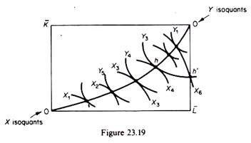
If the production isoquants are concave to the origin the Edge-worth contract curve of production becomes the locus of tangencies (of the isoquants of X and Y) where the output of X is minimum for a given level of Y, and vice versa. Consider figure 23.19, where both sets of isoquants are concave.

Any point on the contract curve FF’ shows the minimum quantity of X for a given quantity of Y. For example, point h shows the combination Y₃ X₄.However, given Y₃ the maximum amount of X is X₆ (at a ‘corner solution’), while X₄ shows the minimum amount of X given Y₃.

We conclude that with concave isoquants the welfare-maximisation condition that the marginal rate of technical substitution of X and Y be equalised (MRTS^X_L,K – MRTS^y_L,K) will result in input combinations that give a minimum of one commodity amount of the other, that is, a configuration which does not maximise social welfare.

10. Increasing Returns to Scale:

Returns to scale are related to the position of the isoquants, not to their shape. Assume that the isoquants are convex. Increasing returns to scale are shown by isoquants that are closer and closer (for output levels which are multiples of the original level) along any ray from the origin to double output the firm needs less than double inputs.

In our simple model we assumed constant returns to scale. We also saw that decreasing returns to scale do not create serious difficulties except, perhaps, with the treatment of the imbalance between total value of the product and total payments to the factors (the product is not ‘exhausted’ by factor payments) within a general equilibrium approach. However, increasing returns to scale lead to serious difficulties.

Now we will discuss the effects of increasing returns to scale:

(a) On the average cost curves of the firm, and

(b) On the curvature of the production possibility curve.

(A) Increasing Returns to Scale and the AC Curves of the Firm:

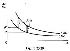
The consequence of increasing returns to scale is that the LAC falls as output increases. We know that when the AC curve falls, the MC curve lies below it. This situation is shown in figure 23.20.

The condition for profit maximisation in a perfectly competitive market is that the firm sets its MC equal to the market price

MC_X = P_x

However, when there are increasing returns to scale, adherence to this rule would lead to losses, since MC < AC. In other words the maximisation of social welfare requires P_x < AC, that is, perpetual losses. But this situation is incompatible with perfect competition: firms which have losses close down in the long run, and the market system collapses.

Increasing returns to scale create another problem, namely the total value of the product is less than total factor payments.

(w. L + r . K) > (P_x . X + P_y .Y)

(B) Increasing Returns to Scale and the Shape of the Production Possibility Curve:

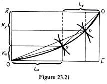
We will continue to assume that the factor intensity (K/L ratio) is different in the two commodities. In particular, the way in which we have been drawing the contract curve of production implies that the (K/L)_x is less than the (K/L)_y. This can be seen from figure 23.21. At point a we have (K/L)_x < (K/L)_y. Similarly at point b we observe that (K/L)_x is less than (K/L)_y. The shape of our contract curve implies that X is less capital intensive than Y.

With different factor intensities, if the increasing returns to scale are not important, the PPC can still be concave to the origin, so that the model is valid. While doubling the inputs in the production of X would more than double the output of X, an increase in X at the expense of Y will, in general, not take place by means of such proportional expansion of factors, because efficient production takes place along the contract curve, and at each point of this curve the K/L ratio of X and Y change; as we have drawn the contract curve of production, labour is-more important relative to capital in producing X, and vice versa for Y.

Thus as the production of X expands, the producers of X will be coerced to use capital in greater proportion to labour. In other words, the K/L ratio in X becomes less ‘favourable’ as the production of X expands. The opposite is true of the K/L ratio in Y as the production of Y declines.

The above argument remains valid if we have unimportant increasing returns to scale in both functions. The PPC will become less curved, but so long as it stays below the diagonal of the Edgeworth box the production possibility curve will be concave, as required for the unique solution of the welfare-maximisation problem. In this ‘mild’ case of increasing returns to scale, with a still concave PPC, the previous maximising rules give the correct result for a maximum social welfare.

Furthermore, the constants embedded in the system retain their meaning as ‘prices’, because they still reflect marginal rates of substitution and transformation. In this case also, the total value of maximum-welfare ‘national’ output (V* = P_x . X + P_y . Y) valued at these ‘shadow prices’ (constants of the system), is still at a maximum.

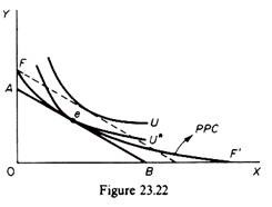
If, however, the increasing returns to scale are strong the production possibility curve will be convex to the origin (figure 23.22). In this case two results are possible, depending on the curvature of the community indifference curves.

(i) If the curvature of the community indifference curves is greater than the curva­ture of the convex production possibility curve, social welfare is maximised at e, where the isovalue-product line AB is tangent to the production possibility curve. The constants implied by the maximum-of-welfare problem retain their meaning as ‘shadow prices’: they still reflect marginal rates of substitution and transformation.

However, maximum social welfare is no longer associated with maximum value-of- output. In fact at point e the value-of-output is at a a minimum. Given P_x/P_y the value of output would be maximised at either F or at F’ (the ‘corners’ of the convex production possibility curve). Thus, if the curvature of the PPC is smaller than that of the community indifference curves, social welfare is maximised, but the value of output is at a minimum.

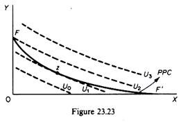
(ii) If, however, the curvature of the PPC is greater than the curvature of the community indifference curves, both social welfare and value of output are mini­mised if we apply the rules of welfare maximisation. In figure 23.23 the production possibility curve FF’ is more convex than the indifference curves (U), and the point of tangency z is a point of both minimum welfare and minimum value of output. Welfare maximisation is attained at point F, a ‘corner tangency’ of the PPC and the highest possible community indifference curve (U₂).

In summary, when the PPC is convex to the origin, the relative curvatures (of the PPC and the community indifference curves) are crucial: tangency points may be either maxima or minima of welfare.

11. Indivisibilities in the Production Function:

If the technology consists of small-scale and large-scale production processes, with large-scale methods having a lower average cost than the small-scale methods, but large-scale methods are indivisible, then perfect competition does not result in a Pareto-optimal allocation of resources, nor to a maximisation of social welfare.

Assume a situation in which perfect competition prevails with a large number of small firms being in equilibrium. Furthermore, assume that the economy has at­tained the equality of the MRPT and the (equalized) MRS of the two commodities among the consumers. Although in this situation (configuration) the three marginal conditions of Pareto optimality are fulfilled, the use of resources is inefficient and social welfare is not maximized if the production methods are indivisible and the small firms cannot take advantage of the lower cost of the large-scale production techniques.

Under these conditions it is obvious that a few large firms, using the more efficient large-scale methods, can produce a greater amount of output with the same total quantities of inputs available in the economy. This means that the small firms produce at a point below the PPC, because, due to the indivisibilities, they cannot make full use of the available technical knowledge. Although the small firms satisfied the marginal condition for efficient production the use of resources was really inefficient in the initial situation: the small firms produced less output with the same amounts of resources.

In conclusion, the existence of indivisibilities is incompatible with the assumptions of perfect competition and the 2 x 2 x 2 welfare model.

From the above examination of the assumptions of the 2 x 2 x 2 model, we may conclude that the model collapses when:

(i) A welfare function does not exist;

(ii) There are externalities in production;

(iii) There are interdependencies in the utility functions;

(iv) There are strong economies of scale, which render the PPC convex to the origin and its curvature is greater than the curvature of the community indif­ference curves;

(v) There are indivisibilities in the production function.