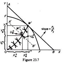
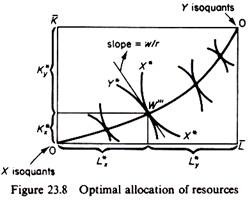
From the bliss point we can determine the optimising (welfare-maximising) values of the ten unknowns of the 2 x 2 x 2 model:
(a) The total quantities of the two products X* and Y*;
(b) The quantities of X* and Y* that will be consumed by the two consumers: X*A, X*B, Y*A, Y*B.
(c) The quantities of capital and labour which will be used in the production of the optimal product-mix, Lx, Ly, Kx, Ky.
ADVERTISEMENTS:
By retracing our steps we will show that the maximum welfare configuration (state) is determinate, in that it yields unique values to the above ten unknowns involved.
The constrained bliss point W* is associated with a unique commodity-mix on the production possibility curve, because W* defines the utility combination U*A U*B → which belongs to a particular utility frontier. → But recall that each utility frontier is derived from a single (unique) point on the production possibility curve.
Thus, assume that the utility possibility frontier, to which U*A U*B belong, corresponds to the unique point W’ on the production possibility curve FF’ in figure 23.7. Point W’ defines the welfare-maximising commodity combination Y*X*.
We next construct the Edge-worth box of exchange with precise coordinates the welfare-maximising levels of outputs Y* and X*. By examining the contract curve 0 W we can locate the one point where the utilities of the two consumers are U*A and U*B. At this point (W” in figure 23.7) the ‘equalised’ slope of the indifference curves of consumers A and B is equal to the slope of the PPC at W. Point W” defines the distribution of X* and Y* between the two consumers (X*A, X*B, Y*A and Y*B in figure 23.7).
Finally, point W on the production possibility curve defines point W'” on the contract curve of the Edgeworth box of production. (The PPC was derived, point by point, from the contract curve of the Pareto-efficient input locus.) In figure 23.8 point W'” is the point of tangency of the isoquants Y* and X* implied by the bliss point. By drawing perpendiculars through W'” we define the amount of capital K and labour L
which will be used in the production of Y* and X*. The welfare-maximising resource allocation is shown by the length of the segments marked by the brackets and denoted by the symbols L*x, K*y and K*y.
In summary, the maximum-welfare configuration is determinate. We have solved (found unique values) for the total outputs, the distribution of these outputs between the two consumers, and for the labour and capital to be used in the production of the welfare-maximising outputs.

