Income Elasticity of Demand: Definition, Measures, Types and Other Details

Another important concept of elasticity of demand is income elasticity of demand. Income elasticity of demand shows the degree of responsiveness of quantity demanded of a good to a small change in income of consumers.

The degree of responsiveness of quantity demanded to a change in income is measured by dividing the proportionate change in quantity demanded by the proportionate change in income.

Thus, more precisely, the income elasticity of demand may be defined as the ratio of the proportionate change in the quantity purchased of a good to the proportionate change in income which induces the former.

Income Elasticity = Proportionate change in purchases of a good / Proportionate change in income

Thus if the proportionate change in purchases or quantity demanded of a good exceeds that of proportionate change in income, income elasticity will be greater than one. For example, if a 2 per cent change in income leads to 5 per cent change in quantity demanded of a good, income elasticity of the demand for the good will be 5%/2%=2.5.

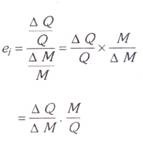
Let M stand for an initial income, AM for a small change in income, Q for the initial quantity purchased demand, AQ for a change in quantity purchased as a result of a change in income and e,- for income elasticity of demand. Then

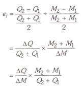
Midpoint formula for measuring income elasticity of demand when changes in income are quite large can be written as:

Income Elasticity, Normal Goods and Inferior Goods:

It is important to note that the value of zero income elasticity of demand is of great significance. Zero income elasticity of demand for a good implies that a given increase in income does not at all lead to any increase in quantity demanded of the good or increase in expenditure on it. In other words, zero income elasticity signifies that quantity demanded o the good is quite unresponsive to changes in income.

Besides, zero income elasticity is significant because it represents a dividing line between positive income elasticity on the one side and negative income elasticity on the other. When income elasticity is more than zero (that is, positive), then an increase in income leads to the increase in quantity demanded of the goods.

This happens in case of normal goods. On the other side there are all those goods which have income elasticity less than zero (that is, negative) and in such cases increase in income leads to the fall in quantity demanded of the goods. Goods having negative income elasticity are known as inferior goods. We thus see that zero income elasticity is a significant value, tor it represents a dividing line between positive income elasticity and negative income elasticity and therefore helps us in distinguishing normal goods from inferior goods.

Income Elasticity, Luxuries and Necessities:

Another significant value of income elasticity is unity. This is because when income elasticity of demand for a good is equal to one, then proportion of income spent on the good remains the same as consumer’s income increases. Income elasticity of unity also represents a useful dividing line.

If the income elasticity for a good is greater than one, the proportion of consumer’s income spent on the good rises as consumer’s income increases, that is, that good bulks larger in consumer’s expenditure as he becomes richer. On the other hand, if income elasticity for a good is less than one, the proportion of consumer’s income spent on it falls as his income rises, that is, the good becomes relatively less important in consumer’s expenditure as his income rises.

A good having income elasticity more than one and which therefore bulks larger in consumer’s budget as he becomes richer is called a luxury. A good with an income elasticity less than one and which claims declining proportion of consumer’s income as he becomes richer is called a necessity.

It should, however, be noted that the definitions of luxuries and necessities on the basis of income elasticity may not conform to their definitions in English dictionary because the dictionary’s luxuries may be necessities and its necessities may be luxuries according to the above definition. But in economic theory it is useful to call the goods with income elasticity greater than one as luxuries and goods with income elasticity less than one as necessities.

Income Elasticity Defined in Terms of Expenditure:

We can also express the income elasticity in terms of changes in expenditure made on the good rather than the change in quantity purchased of the good as a result of a change in income. It should be noted that expenditure is equal to the quantity purchased of the good multiplied by the price of the good. If Q is the quantity purchased of the good and P the price of the good, the expenditure made on the good will be equal to QP.

As defined above,

Multiplying the numerator and denominator by P, we get

Now,as explained above, Q.P is the expenditure made on the good and ∆ Q. P is the change in expenditure made as a result of change in income. Let E stand for the expenditure made on the good.

Then the above equation will become:

It is important to note that the value of zero income elasticity of demand is of great significance. Zero income elasticity of demand for a good implies that a given increase in income does not at all lead to any increase in quantity demanded of the good or increase in expenditure on it. In other words, zero income elasticity signifies that quantity demanded of the good is quite unresponsive to changes in income.

Besides, zero income elasticity is significant because it represents a dividing line between positive income elasticity on the one side and negative income elasticity on the other. On the one side, when income elasticity is more than zero (that is, positive), then an increase in income leads to the increase in quantity demanded of the good.

This happens in case of normal goods. On the other side of zero income elasticity are all those goods which have income elasticity less than zero (that is, negative) and in such cases increase in income will lead to the fall in quantity demanded of the goods. Goods having negative income elasticity are known as inferior goods. We thus see that zero income elasticity is a significant value, for it represents a dividing line between positive income elasticity and negative income elasticity and therefore help us in distinguishing normal goods from inferior goods.

Another important value of income elasticity is the reciprocal of proportion of consumer’s income spent on a good, that is 1/K_x where K_x stands for the proportion of consumer’s income spent on a good X. The value of 1/K_x for the income elasticity of demand seems to be significant because when income elasticity for a good equals 1/K_x, then the whole of the increase in consumer’s income will be spent on the increase in quantity purchased of the good X.

Proof:

It is easy to show that when whole of the increase in income is spent on any good X, then income elasticity is equal to the reciprocal of the proportion of income spent on the good, that is, 1/K_x.

We know that e_i = M/E. ∆E/∆M

Suppose the whole of the increase in income (∆M) is spent on the good X, then change in expenditure (∆E) on the good X would be equal to ∆M, price of good X remaining the same. Substituting ∆ M for ∆ E in the above measure of income elasticity, we get

It may be further noted that if income elasticity of demand for a good is greater than 1/K_x, then more than the increase in consumer’s income would be spent on the good and vice versa.

Measuring Income Elasticity at a Point on an Engel Curve:

An Engel curve shows the relationship between quantity demanded of a good and level of consumer’s income. Since with the increase in income normally more quantity of the good is demanded, Engel curve slopes upward (i.e. it has a positive slope).Though Engel curve for normal goods slopes upward but it is of different shape for different goods.

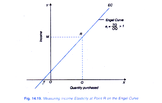
It is convex or concave, depending on whether the good is a necessity or a luxury. In case of an inferior good for which income effect is negative, that is, less is demanded when income rises. Engel curve is backward bending. We will first explain howincome elasticity is measured at a point on a linear Engel curve EC in Fig. 14.19 which is sloping upward.

It is required to measure income elasticity at point R on this Engel curve. It will be seen that at point R, the quantity of a good OQ is purchased at the income level OM. Let us extend the Engel curve EC downward so that it meets the X-axis at point T.

e_i = ∆Q/∆M . M/Q …(i)

∆Q/∆M is the reciprocal of the slope (∆ M/∆Q) of the Engel curve EC. Rewriting the income elasticity measure we have

e_i = 1/ ∆M / ∆Q . M/Q

It will be seen from the Engel curve EC in Figure 14.19 that at point R on it, its slope (i.e. ∆M/∆Q equals RQ/TQ and level of income (M) equals RQ and quantity purchased at this income level equals OQ. Substituting these in (ii) above we have

e_i = 1 / ∆M / ∆Q . M/Q = 1 / RQ / TQ. RQ/OQ

= TQ/RQ. RQ/OQ = TQ/OQ

Thus, income elasticity at point R on the Engel Curve EC in Figure 14.19 can be obtained by measuring the lengths TQ and OQ and dividing the former by the latter. Since in Figure 14.19 TQ is larger than OQ, income elasticity at point R is greater than one (However, the exact magnitude of income elasticity can be found by actually dividing TQ by OQ). We therefore conclude that if Engel curve on being extended downward meets X-axis to the left of the point of origin income elasticity will be greater than one.

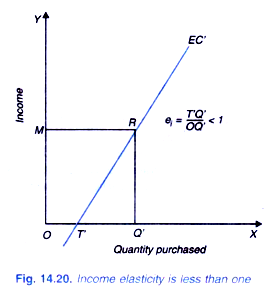
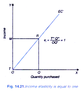
In Figure 14.20 at point R on Engel curve EC, income elasticity is equal to TQ’/OQ. Since TQ’ is less than OQ’, income elasticity will be here less than one. We therefore conclude that if Engel curve when extended downward meets the X-axis to the right of the point of origin, income elasticity will be less than one. In Figure 14.21 Engel curve when extended meets the point of origin, income elasticity at point R is equal to one (TQ/OQ in Figure 14.21 equals one).

Measuring Income Elasticity at a Non-Linear Engel Curve:

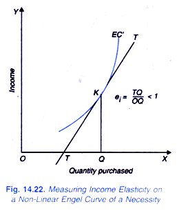
If Engel curve is non-linear as is usually the case in the real world, the income elasticity can be measured at a point on the Engel curve by drawing a tangent at the point and extending it to meet the X-axis. Suppose we are required to measure income elasticity at K on the non­linear Engel curve EC drawn in Figure 14.22 where at income level OM, quantity OQ is being demanded. We draw a tangent TT at point K and extend it to meet the X-axis at point T.

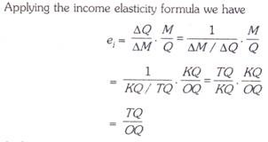
Applying the income elasticity formula we have:

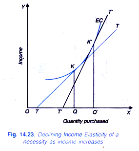
A glance at Figure 14.22 shows that the length TQ is less than OQ. Therefore, income elasticity at point K on the non-linear and outwardly convex Engel curve of a necessity is less than one. Income elasticity will vary at different levels of income. And further in the case of Engel curve having outwardly convex slope, the income elasticity of the good is declining as income increases as will be seen from Fig. 14.23.

This indicates the responsiveness of demand to increase in income falls as a consumer becomes richer. Non-linear convex Engel curve represents the case of a necessity which accounts for a smaller proportion of income of the richer families as compared to the poor people.

Engel Curve and Income Elasticity: Necessities, Luxuries, and Inferior Goods:

As stated above, the Engel curve shows the relationship, between quantity demanded of a good and changes in levels of consumer’s income. An Engel curve can take various shapes depending upon whether the good is a necessity, luxury or an inferior good.As explained above, in case of a necessity, income elasticity is positive but less than unity and the quantity demanded increases less than proportionately to increase in income. Therefore, the Engel curve of a necessity will be convex as shown in Figure 14.23.

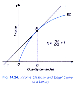
On the other hand, in case of luxuries, income elasticity is greater than one. As income increases the consumer spends more than proportionate increase in income on them. Income elasticity of a luxury good increases at higher levels of income. Therefore, for luxuries, Engel curve is concave as shown in Figure 14.24. Finally, in case of inferior goods, income elasticity is negative and consumer’s quantity demanded of these goods declines as their income increases.

Engel curve bends backward and has a negative slope beyond a certain level of income as illustrated in Figure 14.25. It will be observed from figure 14.25 that an inferior good behaves like a necessity in the initial ranges of income and therefore the slope of its Engel curve is initially positive, and only after a particular level of income, it bends backward.

Thus, in Figure 14.25, it is only after point B that Engel curve bends backward indicating that beyond this point if income increases, quantity demanded of the good declines. Therefore, if we calculate income elasticity at point R on the backward-bending portion using the income elasticity measure TQ/OQ, we get a negative TQ distance over the positive distance OQ. Hence e, = TQ/OQ < 0.

Income Elasticity and Proportion of Income Spent:

There is a useful relationship between income elasticity for a good on the one hand and proportion of income spent on it.

The relationship between the two is described in the following three propositions:

1. If proportion of income spent on the good remains the same as income increases, then income elasticity for the good is equal to one.

2. If proportion of income spent on the good increases as income increases, then the income elasticity for the good is greater than one.

3. If proportion of income spent on the good decreases as income rises, then income elasticity for the good is less than one.

We give below proofs of the above three propositions.

Theorem 1: If proportion of income spent on a good remains the same as income increases, income elasticity for the good is equal to one.

Let E stand for the income spent on a good and M for a level of income. The proportion of income spent will then be E/M. If the income increases by ∆M and as a result expenditure on the good rises by ∆E, new proportion of income spent on the good will be E + ∆E/M + ∆M. Now, if proportion of income spent on the good remains the same as income increases, then

Since EM occurs on both sides of the equation, it will cancel out. Therefore, M ∆E = E ∆ M

Or ∆E/∆M. M/E = 1

But ∆E/∆M. M/E is an expression for income elasticity of demand. We therefore conclude that when with the change in income, proportion of income spent on a good remains constant income elasticity for it is equal to unity (e_{ = 1). Likewise, we can prove the other two theorems.

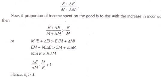
Theorem 2: If the proportion of income spent on the good rises as income increases, the income elasticity is greater than unity.

As stated above, E/M is the proportion of income spent on a good, E stands for expenditure made on the good and M for consumer’s income. Suppose income increases by AM and as a result the income spent on the good rises by AE, the new proportion of income spent on the good will equal to

We, therefore, conclude that if proportion of income spent on the good increases as income increases, income elasticity is greater than one.

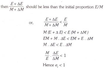
Theorem 3. If the proportion of income spent on the good decreases as income increases, income elasticity is less than one.

If the proportion of income spent on a good has to decrease with the increase in income, then

We, therefore, conclude that when proportion of income spent on the good falls as income increases, income elasticity is less than unity.

Sum of Income Elasticities, Budget Constraint and Expenditure:

Increase in income can be spent on a number of goods and services demanded by a consumer. Given the budget constraint, when some part of an increase in income is not spent on a good, it must be spent on other goods and services, assuming that there is no saving and borrowing by the consumer. From this, a relationship can be derived which shows that the sum of income elasticities for all goods and services must be unity and further that income elasticity of demand for a good depends on income elasticity of other goods and services.

Suppose that consumer has an income equal to M and further that all his income is spent on two goods X and Y. Let P_x and P_y represent the prices of two goods X and Y respectively. Let income increases by AM and as a result quantities purchased of two goods increase by AQ_x and ∆Qy. Then, budget constraint can be written as

∆M = P_x . ∆ Q_x ∆ + Py . ∆Q_y

Dividing both sides of the budget equation by ∆M we have

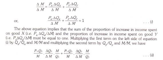
The above equation implies that the sum of the proportion of increase in income spent on good X (i.e. P_x ∆Q_x /∆M) and the proportion of increase in income spent on good Y (i.e. P_y∆Q_y /∆M) must be equal to one. Multiplying the first term on the left side of equation (i) by Q_x/Q_x and M/M and multiplying the second term by Q_y/Q_y and M/M, we have

It will be seen that the term P_x Q_x /M represents the proportion of income spent on good X and ∆Q_x/ ∆M . M/Q_x the income elasticity of demand for good X. Similarly, term P_y Q_y /M is the proportion of income spent on goods Y, and the term ∆P_y / ∆M. M/Q_y the income elasticity of demand for good Y.

Using K_x to denote proportion of income spent on good X, K_y for the proportion of income spent on good Y, e_xi for income elasticity of demand for good X, and e_yi for income elasticity of demand for good Y, then from equations (i) and (ii) we have

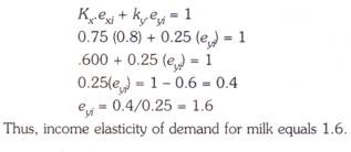
K_xe_xi + K_y e_yi = 1

The above equation reveals that the weighted sum of the income elasticities of demand for all goods (weights being the proportion of income spent on goods) must equal unity. This for example, means that when income increases by 10 per cent, the budget constraint requires that purchases or consumption of goods as a whole must also increase by 10 per cent.

If there is a 10 per cent increase in income, if the consumption of some goods increases by less than 10 per cent, the consumption of others must increase by more than 10 per cent so that the increase in income must somehow be spent on the goods. That is, the increase in consumption of goods whose income elasticity of demand is less than one must be offset by increase in consumption of others for which income elasticity of demand is greater than one.

Thus, on the average, consumption of goods must increase by the same proportion as income. If there are two goods X and Y, then the above equation K_x e_xi + K_ye_yi = 1 must hold. This equation implies that given the two goods on which a consumer spends his income, if we know the proportion of income spent of one good and the income elasticity for that good, we can calculate the income elasticity of demand for the other good.

Numerical Example:

Assume that there are two commodities, rice and milk. If rice accounts for 75% of the budget and has income elasticity equal to 0.8, what would be the income elasticity of milk?

Let us call rice as commodity X and milk as commodity Y

Thus, income elasticity of demand for milk equals 1.6.

Importance of Income Elasticity for Business Firms:

The concept of income elasticity is important for decision making both by business firms and industries. First, the firms producing products which have a high income elasticity have great potential for growth in an expanding economy. For example, if for a firm’s product income elasticity of demand is greater than one, it means that it will gain more than proportionately to the increase in national income.

Thus firms which are producing products having high income elasticity are more interested in forecasting the level of aggregate economic activity (i.e., level of national income) because the demand for their products greatly depends on the level of overall economic activity.

Further, as seen above, the demand for luxuries is highly income elastic. Therefore, the demand for luxuries fluctuates very much during different phases of business cycles. During boom periods, demand for luxuries increases very much and declines sharply during recessionary periods.

On the other hand, the demand for products with low income elasticity will not be greatly affected by the fluctuations in aggregate economic activity. During booms the demand for these products will not increase much and during recessions it will not decrease sharply. Therefore, the firms with low income elasticity for their products would not be much interested in forecasting future business activity. Remember it is generally necessities for which demand is not much income elastic.

However, there is one good thing for the firms which produce goods having low income elasticity. They are to a good extent recession-proof. In the periods of recession, their incomes do not fall to the extent of decline in aggregate income. Of course, to share the benefits of increasing national income firms currently producing products with low income elasticity would try to enter the industries demand for whose products is highly income elastic as this would ensure better growth opportunities.

The knowledge of income elasticity of demand also plays a significant role in designing marketing strategies of the firms. If income of people is an important determinant of demand for a product, the firms producing products with high income elasticity of demand will be located in those areas or set up their sales outlets in those cities or regions where incomes are increasing rapidly. Besides, the firms will direct their advertising campaigns and other sales promotion activities to those segments of people whose income is high and also increasing rapidly. This is to ensure higher growth of sales of their products.

The concept of income elasticity of demand shows clearly why farmers’ income do not rise equal to that of urban people engaged in manufacturing industries. Income elasticity of demand for agricultural products such as food grains is less than one.

This implies that it is difficult for the farmers’ income from agriculture to increase in proportion to the expanding national income. Thus farmers’ income cannot keep face with the urban people who derive their income from industries producing goods with high income elasticity of demand.

Some Numerical Problems on Income Elasticity:

Problem 1.

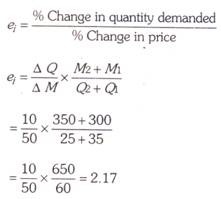
If a consumer’s daily income rises from Rs. 300 to Rs. 350, his purchase of a good X increases from 25 units per day to 35 units, find income elasticity of demand for X.

Solution.

Change in quantity demand (∆Q) = (Q₂ = Q₁) = 35 – 25 = 10

Change in income (∆M) = M₂ – M₁ = 350 – 300 = 50

Income elasticity of demand in this case is 2.17.

Problem 2.

Suppose demand for cars in Bombay as a function of income is given by the following equation:

Q = 20,000 + 5M

Where Q is quantity demanded. M is per capita level of income in rupees.

Find out income elasticity of demand when per capita annual income in Bombay is Rs 15,000.

Solution.

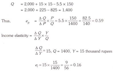
Income elasticity (e_i) = ∆ Q / ∆ M. M/Q

In order to obtain income elasticity, we have to first find out quantity demanded (Q) at income level of Rs 15,000. Thus.

Q = 20,000 + 5 x 15,000 = 95,000

It will be seen from the given income demand function that coefficient of income (M) is equal to 5. This implies that ∆Q/∆M = 5. With this information we can calculate income elasticity.

Problem 3.

The following demand function for readymade trousers has been estimated:

Q = 2,000 + 15y – 5.5P

Where Y is income in thousands of rupees, Q is the quantity demanded in units and P is the price per unit.

(a) When P = Rs 150 and Y = 15 thousand rupees, determine the following

1. Price elasticity of demand

2. Income elasticity of demand

(b) Determine what effect a rise in price would have on total revenue.

(c) Assess how sale of trousers would change during a period of rising incomes.

Solution.

(a) Coefficient of P, i.e., ∆ Q / ∆ P = 5.5

Price elasticity of demand ∆ Q / ∆ P = 505 x 150/Q

Let us first find out the quantity demanded (i.e., Q at the given income (Y = 15 thousands) and given price (P = Rs 150 per unit).

Substituting the values of income and price in the given demand function, we have:

(b) Since price elasticity of demand for trousers is less than one, rise in price would cause increase in total revenue.

(c) Since income elasticity of demand for trousers is less than one, trousers are a necessity and therefore the increase in income of the people will lead to less than a proportionate increase in their sales.