In this article we will discuss about the cobweb model to study market equilibrium.
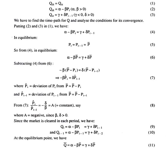
Suppose that in the market for a single good, the supply and demand equations for period t are given by:
where the symbols have their usual meanings. It is assumed that the price is set in each period to clear the market. Note here that this is a model with lagged supply— as is evident in eqn. (4.25), this period’s supply depends upon the previous period’s price or this period’s price influences the supply of the following period.
ADVERTISEMENTS:
Since production takes time, the adjustments on the supply side may not be instantaneous, but may be perceived in the market only after a period of time. Agricultural commodities often provide good examples of lagged supply.
Now, if the slope of the supply function (β1) is positive and that of the demand function (β2) is negative, then to examine the convergence or divergence of the current price towards or away from the equilibrium level. This model is known as the Cobweb model because, the path taken by the observed price and quantity resembles a cobweb.
Now go into the question of convergence or otherwise of the current price towards the equilibrium price. Since it is assumed here that the price is set in each period to clear the market,
St = Dt ……(4.27)
ADVERTISEMENTS:
To study the model’s behaviour out of equilibrium if β1 > 0 and β2 < 0.
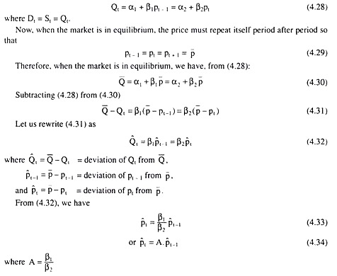
Substitute (4.25) and (4.26) in (4.27), and we obtain:
ADVERTISEMENTS:
ADVERTISEMENTS:
ADVERTISEMENTS:
Equation (4.34) is a first order difference equation and it gives us t as a function of
t−1, β1 and β2 being given and constant. The solution for
at any time t is given by
The solution (4.35) may be obtained in the following way:
ADVERTISEMENTS:
3 = A.
2 = A3.
0 and so on, in this way
t = At
0.
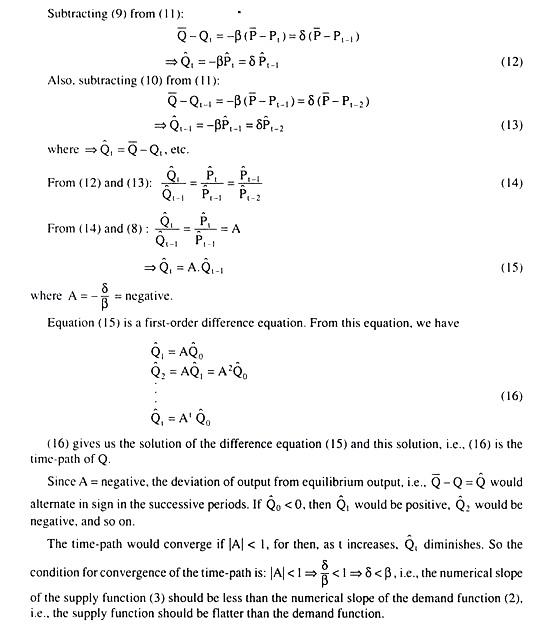
Equation (4.35) gives the general solution for the linear Cobweb model as given by equation (4.25) − (4.27). This gives t, given the slopes of the demand and supply functions and the values of
0. This value of
0 = (
– p0) is called the initial arbitrary disturbance which can take on any sign and magnitude that would like to give it.
The original 0 ≠ 0 might have been brought about by a shift in either the demand or the supply curve so that
0 represents the difference between the new and the old equilibrium prices.
If β1 > 0 and β2 < 0, i.e., the supply function slopes upwards and the demand function slopes downwards, A to be negative. Thus, At will alternate in sign, being negative in odd-numbered periods and positive in even-numbered periods.
ADVERTISEMENTS:
This proves that with the normal-shaped demand and supply curves, the Cobweb will always produce a two-period oscillation with the actual price (pt) being alternately above and below the equilibrium price () . If these oscillations will converge on to, or, diverge from,
. But before doing this, note that in the demand-supply curve diagrams, generally measure quantity along the horizontal axis and price along the vertical axis. In that case, the slopes of the supply and demand curves would be, respectively, the reciprocals of the slopes of the supply and demand functions (i.e., β1 and β2).
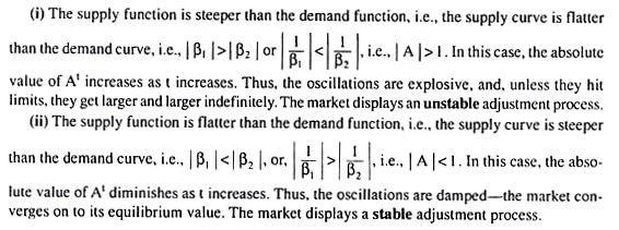
Also note that if β1 is positive, then the slope of the supply curve, 1/β1, would also be positive and if β2 is negative, then the slope of the demand curve, 1/β2, would also be negative. Now, even if the supply and demand functions and curves have their normal slopes (i.e., positive and negative respectively), then also to consider three cases in respect of convergence or divergence.
ADVERTISEMENTS:
It is obtained from the above analysis that the linear Cobweb model displays negative feedback
ADVERTISEMENTS:
Whenever price is above equilibrium, it falls in the next period, and whenever price is below equilibrium, it rises in the next period; but the adjustment is always too much and so the equilibrium price is always overshot.
In the stable case, the overshot gets smaller and smaller so that the equilibrium price is approached. On the other hand, in the unstable case, each overshot is larger than the previous one, so that the actual price diverges from equilibrium more and more as time passes.
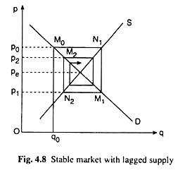
From the above analysis, the negative feedback is obtained, although a necessary condition for stability, is not a sufficient condition. Now attempt a diagrammatic representation of the Cobweb model in Fig. 4.8. Suppose that initially the supply of the good concerned has fallen short of the equilibrium amount because of some disturbance such as drought or flood. Let the initial supply be q0.
ADVERTISEMENTS:
This amount would be demanded in the initial period if the price be p0. At p = p0, the consumers demand P0M0 and this quantity equals the initial supply. That is, p0 is the market-clearing price in period 0.
In the Cobweb model, this period’s price influences the next period’s supply. That is why the price, p0, of the initial period (period 0) determines the supply of period 1, which is P0N1. In other words, the price p0 induces the entrepreneurs to supply p0N1 in period 1.
Now the buyers would demand this quantity, p0N1 only when price falls to p1 in period 1. Therefore, p1 is the market clearing price in period 1. However, the price P1 in period 1 induces the producers to supply the quantity of p1N2 in period 2.
In this way, the process continues indefinitely, producing a Cobweb pattern. See in Fig. 4.8 that the price level fluctuates, being higher than the equilibrium price pe in one period and lower than pe in the next period, but converges to the equilibrium level at the point of intersection of the demand and supply curves.
This convergence would be obtained if the demand curve is flatter than the supply curve.
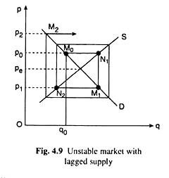
In Fig. 4.9, the same process as obtained in Fig. 4.8, operates but the price fluctuations tend to become larger and larger and the market is subject to explosive oscillations, i.e., here price diverges away from equilibrium and the market is unstable. As already obtained, this will be the case if the demand curve is steeper than the supply curve.
Example 1:
Consider the following Cobweb model (the notations having their usual meanings):
Find the time-path of Q and analyse the conditions for its convergence.
Solution:
The equations of the given Cobweb model are
Example 2:
Consider the following two competitive markets:
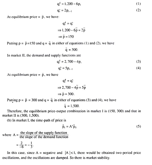
Market I : (i) qdt = 1200 − 6pt; (ii) qst = 2pt−2,
Market II: (i) qdt = 2700 − 4p, ; (ii) qst = 5pt-1
where qdt and qst refer to demand and supply functions and t refers to the time period.
(a) Discover the equilibrium price and quantity in both markets.
(b) Consider the stability of the adjustment to a disturbance in each market.
(c) Draw a time series graph for p in the first five periods following a disturbance that moves price 200 units above its equilibrium in market I and 20 units below it in market II.
(d) The explosive oscillations in one market cannot go on increasing indefinitely. What economic limits to oscillation are finally reached?
Solution:
(a) The demand and supply function for market I:
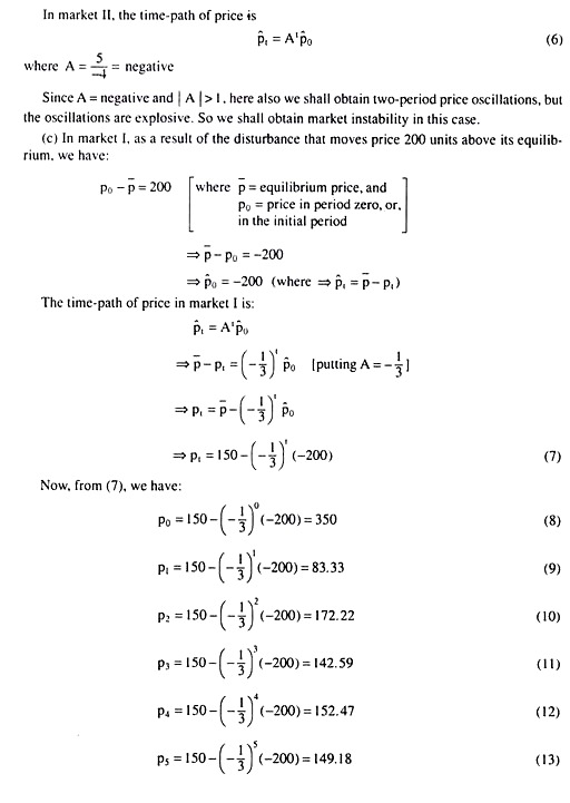
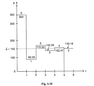
The price-figure in market I in period 0 (zero) and in the next five period are obtained in (8) – (13), respectively. On the basis of these values, the time-series graph for price in market I has been drawn in fig. 4.10.
In market II, because of the disturbance that moves price 20 units below its equilibrium:
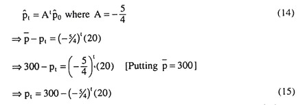
Now, the time-path of price in market II is:
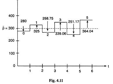
Putting t = 0, 1, 2, 3, 4, and 5 in (15), the price-figures for these period is obtained as: p0 = 280, p1 = 325, p2 = 268.75, p3 = 339.06, p4 = 251.17 and p5 = 361.04. On the basis of these values, the time-series graph for price in market II is obtained as shown in fig.4.1
(d) According to our assumptions, the market price of a good does not have an upper limit, tort it has a lower limit which is zero. So economic limits to explosive oscillations in market II are reached when price, ultimately, oscillates down to zero or less than zero, and that occurs in the 14th period. The following way is obtained.
It is evident from (15) that pt becomes less than p̅ = 300 in even periods, and so, let us remember, pt would approach zero, or, a negative value in even-numbered periods. But let us,
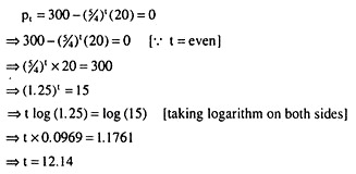
for the time being, put pt = 0 in (15) assuming A = 5/4 which is positive and greater than 1, and, then:
What will be obtained here is that if t were a continuous variable and if assumed A to be positive and greater than 1(= 5/4), then p would monotonically move downwards (i.e., without any oscillation) and would become zero (0) in period t = 12.14 (approx.). That is, in period t = 12, p would still be positive (it can be calculated as, p = 9).
Therefore, in our discrete time case, p in t = 13, would oscillate up to p13 which is above = 300. And the process of oscillation comes to an end in period t = 14 because, now p would go down to become negative [it can be calculated as, p14 = − 154.6 (approx..).]
Example 3 :
Consider the following markets which are characterized by lagged supply response:
(a) Dt = 40 – 10 Pt ; St = 2 + 9Pt−1
(b) Dt =30 – 5 Pt ; St = 20 − Pt−1
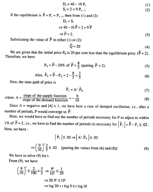
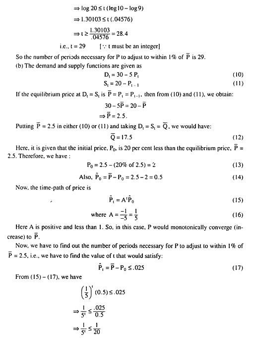
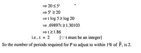
Determine equilibrium price and quantity for each market. Assume an initial price 20% below the equilibrium price for each market, and determine the number of periods necessary for each price to adjust to within 1 % of equilibrium.
Solution:
(a) The demand and supply functions are:
