Aggregate Demand Curve and Aggregate Supply

In this article we will discuss about the Aggregate Demand Curve and Aggregate Supply.

Aggregate Demand Curve:

The aggregate demand curve is the first basic tool for illustrating macro-economic equilibrium. It is a locus of points showing alternative combinations of the general price level and national income. It shows the equilibrium level of expenditure changes with changes in the price level.

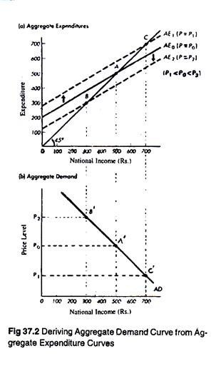
Fig. 37.2 shows how the AD curve is derived by shifting the AE curves. In Fig. 37.2(a) we show three AE curves corresponding to three different price lev­els. In fact, each AE curve corresponds to a particu­lar price level.

Here the initial equilibrium occurs at point A at which the 45° guideline interests the AE₀ line (with price P₀). In this case equilibrium income and expenditures are Rs. 500 crores. If the general price level falls to P₀, the AE line shifts upward to AE₁ (for reasons explained above).

Now a new equi­librium is established at point C, at which national income equals Rs. 700 crores. If, on the other hand, the general price level rises from P₀ to P₂, the AE line shifts downward to AE₂. Now a equilibrium is established at point B, with national income equal to Rs. 300 crores.

In the lower part of the diagram, i.e., in Fig. 37.2 (b) we plot the price level on the vertical axis and national income (in Rs. crores) on the horizontal axis. If we move vertically from points A, B and C in the top half of the diagram, we are able to locate three corresponding points in the lower half of the diagram (A’. B’ and C’).

The locus of these three points is the aggregate demand curve AD. The AD curve is a locus of all of the combinations of the price levels and corresponding equilibrium levels of income and aggregate expenditure.

The AD curve, like the ordinary demand curve of micro-economics is downward sloping for an obvi­ous reason. When the price level decreases aggregate expenditures rise. The converse is also true. In other words, there is an inverse relation between the general price level and the level of aggregate expenditure.

In micro-economics we noted that the demand curve of a normal goods (say X) is downward sloping largely due to substitution effect (and partly due to income effect). If the price of X falls, X becomes relatively cheap.

As a result consumers will buy more X and less of other goods (even when the prices of other goods remain constant). In other words, the demand curve of X is downward sloping due to a change in relative price. As the price of X falls, the quantity of X demanded falls too, all other prices of X the price of Y, price of Z, etc.) remaining unchanged.

However, while deriving the AD curve we show the general price level, i.e., the price level for the en­tire economy on the vertical axis. Here the question of changes in relative price does not arise. Instead a price level change here implies that, on average, all prices in the economy move up or down.

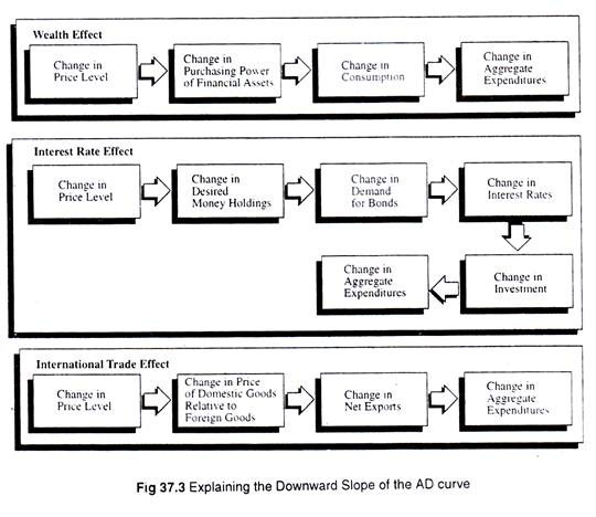
Since there is no change in relative price, the possibility of substi­tution among domestic goods is not considered here. In fact, the negative slope of the AD curve is the com­bined result of three effects, viz., the wealth effect, the interest rate effect, and the international trade effect (see Fig. 37.3).

Shifts in Aggregate Demand:

The AD curve shows equilibrium values of ag­gregate expenditure at different price levels. While deriving this curve from the aggregate expenditure lines we hold all other variables, viz., the non-price determinants of AD such as expectations, foreign in­come, price levels, and government policy, constant.

Should there be a change in any of these variables, the AD curve will shift to a new position. We may now consider possible shifts of the AD curve due to changes in these ‘other things’.

Expectations:

Consumption and investment spending are af­fected by people’s expectations about the future. Con­sumers are sensitive to their expectations of future incomes, prices and wealth.

If, for instance, people expect national and per capita incomes to rise in fu­ture (as in quite normal in the expansionary phase of the business cycle), they will increase their consumption today. Similarly business people are also guided by expectations about the future.

Investment expen­diture largely depends on the marginal efficiency of capital (MEC) which is the expected rate of return on new investment. As J.M. Keynes has put it, “The amount of current investment will depend, in turn, on what we shall call the inducement; and the in­ducement to invest will be found to depend on the relation between the schedule of marginal efficiency of capital and the complex of interest rates on loans of various maturities and risks.”

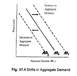
If MEC is likely to in­crease due to technological progress or any other rea­son, more investment is likely to take place in plant, equipment and machinery. In either case the AD curve will shift to the right, say, from AD₀ to AD₁, as shown in Fig. 37.4. Such an increase in aggregate demand implies that at every price level, equilibrium aggregate expenditure are higher than before.

If, on the other hand, people expect a recession in not too distant a future, they will tend to curtail their current consumption and save so as to be able to protect themselves from possible job losses or a forced cutback in hours worked. As consumption falls, ag­gregate demand falls.

This means that the AD curve shifts to the left, from AD₀ to AD₂ .This simply means that at every price level along AD₂, desired expenditures are less than they are along AD₀. The same consequence will follow if investment expendi­ture falls. This will happen when profits are expected to fall, as during depression or recession.

Foreign Income and Price Levels:

The exports are autono­mous (i.e., independent of national income). But if foreign income increases, exports will rise. We may now analyse the effect of changes in the level of foreign prices, i.e., the impact of prices in the rest of the world on the net exports of the domestic economy.

When foreign income increases foreigners spend more. And a portion of this increased spending is on domestic goods. If, for example, USA’s national income rises, a portion of the increased income will be spent on Indian goods (if, however, India is having a trading relation with the USA).

If India’s exports increase, aggregate demand rises. A fall in foreign income will have an exactly opposite effect. When foreign income falls, foreign spending falls, including foreign spending on Indian goods. The end result is a fall in India’s net export and a consequent fall in aggregate demand.

What, then, is the relation between the interna­tional trade effect and the slope of the aggregate de­mand curve? When domestic prices rise, domestic goods become more expensive in relation to foreign goods. This reduces India’s exports. So with a rise in the domestic price level, India’s net exports fall. The same logic applies to changes in the level of foreign prices.

As have been explained by Boyes and Melvin, “If foreign prices rise in relation to domestic prices, domestic goods become less expensive relative to for­eign goods and domestic net exports increase. So do­mestic aggregate demand rises as the level of foreign prices rises. When the level of foreign prices falls, domestic goods become more expensive relative to foreign goods, causing domestic net exports and ag­gregate demand to fall.”

Government Policy:

Government policy also exerts considerable in­fluence on the economy and causes the AD curve to shift. If the government increases the money supply and, as a result, the price level begins to rise, people will try to protect their living standard by spending more and saving less.

As a result the AD curve will shift to the right, which again means that equilib­rium aggregate expenditure increases at every price level. If, on the other hand, the government imposes additional taxes on individuals and companies, both consumption spending and investment expenditure will fall. This will lead to a leftward shift of the AD curve. A government subsidy will have an opposite effect.

1. The AD curve shows the equilibrium level of de­sired expenditure at alternative price levels.

2. The wealth effect, the interest rate effect and the international trade effect are to be combined to explain why the aggregate expenditure curve shifts with changes in the general price level.

3. The AD curve shifts due to changes in non-price determinants viz., expectations of consumers and investors, foreign income and price levels, government policy.

Aggregate Supply:

The aggregate supply curve shows the various quantities of national output (GNP) produced or in­come (GNI) generated at different price levels. Like the ordinary supply curve for an individual commod­ity the aggregate supply curve also slopes upward from left to right. Different factors explain the up­ward slope of the AS curve.

In micro-economics, we noted that when the price of a single good rises (the prices of other goods remaining the same) producers will be willing to offer a larger quantity of the com­modity for sale.

Thus the upward slope of the supply curve of an ordinary commodity is explained by a change in relative price. But while analysing aggre­gate supply, we look at the general price level (or the overall price index which is a weighted average of all prices).

This means that we have now to analyse how the amount of all goods and services produced changes with changes in the level of prices. The di­rect relationship between prices and national output has to be explained by the effect of changing prices on profits. In this context changes in relative price have no role to play.

Aggregate Production and the Price Level:

Along the aggregate supply curve, we hold ev­erything except the price level and output constant. Here the price level is the price of aggregate output (GNP). We also assume that costs of production do not change in the short run even when there are price changes.

If the price level increases but the cost of produc­tion remains unchanged business profits will go up. As profits rise, business firms will be able to produce more output. This means as prices rise, supply will increase (because producers will be willing to offer a larger quantity for sale).

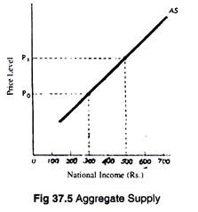
The result is the positively sloped aggregate supply curve as shown in Fig. 37.5. As the price level rises from P₀ to P₁ the volume of output increases from Rs. 300 to Rs. 500. The higher the price, the larger the profits, ceteris paribus, and the larger the volume of production in the macro- economy. The converse is also true. Falling prices and profits give producers the signal to produce less.

The above supply curve is a short-run supply curve. It is drawn on the basis of the assumption that costs of production remain unchanged for the period under consideration. However, costs change in the long run, in which case the upward sloping short-run supply curve of the type shown in Fig. 37.5 will no longer be relevant.

Shifts in Aggregate Supply:

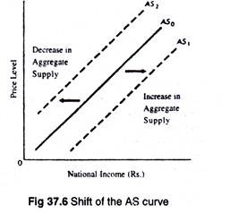
The aggregate supply curve may shift to the right or to the left as shown in Fig. 37.6. Such shifts occur due to changes in non-price determinants of aggre­gate supply, viz., factor prices (such as wage rates, costs of raw materials, etc.), technology and expecta­tions of producers.

Factor Prices:

When commodity prices rise, fac­tor prices do not rise immediately. As a result, cost of production remain unchanged for some time. A rise in commodity prices initially stimulates production. However, when all firms attempt to produce more at the same time, factor prices rise.

This is reflected in the cost of production of each firm. When costs rise in response to the rise in prices the AS curve shifts to the left from AS₀ to AS₂ in Fig. 37.6, (which is comparable to decrease in supply studied in micro­economics). Here, at any given price level, firms pro­duce less output.

The converse is also true. When factor prices (such as wage rates, interest rates and costs of raw materials) fall the AS curve shifts to the right from AS₀ to AS₁ in Fig. 37.6. This means that at any given level of price, firms will produce more output.

A related point may also be noted here. Since here we measure the general price level (which is the weighted average of all prices) only those change in resource prices (such as changes in oil prices) will have an impact on the AS curve.

Technology:

Technological progress has the ef­fect of raising the productivity of existing resources. It thus reduces costs of production and shifts and AS curve to the right, from AS₀to AS₁ in Fig. 37.6. As new technology is adopted, the amount of output that can be produced by each unit of input increases, moving the aggregate supply curve to the right.

Expectations:

If, for some reason, such as in­creased consumer demand, or a policy of tax cut, or growing urbanisation (in the wake of economic development), business people expect profits to rise in future they will step up production. This means that they will be offering larger quantities for sale at the same price levels and the AS curve will now shift to the right.

The Actual Shape of the AS Curve:

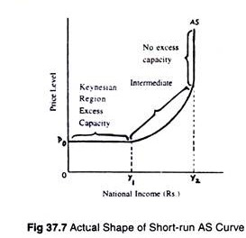
The AS curve does not really look like the lines shown in Figures 37.5 and 37.6. Rather Fig. 37.7 is a correct picturisation of the AS curve. And this curve has three distinct regions.

At relatively low levels of the national income (below Y₁) the AS curve is hor­izontal at the fixed price level P₀. This is known as the Keynesian region. It is that portion of the AS curve at which prices are fixed because of unemploy­ment and excess capacity at these levels.

This Shape of the short-run AS curve are normally observed dur­ing depression and unemployment which means out­put (GNP) can be expanded with rise in the general price level. As output crosses the critical minimum level (Y₁), in the intermediate range the AS curve begins to slope upward, which means that along with output, prices also rise.

This rise in the price level is essential to induce further increases in output. Fi­nally, at the potential (full employment) output level Y₂ the economy is producing its maximum capacity output. In such a situation increased prices have no output effect. Here the AS curve is a vertical straight line, as shown in Fig. 37.7.

The Long-Run Aggregate Supply Curve:

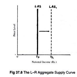
The long-run AS curve is a vertical straight line at the potential level of national income (Y_p) like the one shown in Fig. 37.8. Such a supply curve indicates that there is no relationship between the changes in the price level and the quantity of the output produced. This does not, however, mean that the economy is forever fixed at the current level of potential national income or GNP.

Over an extended period of time, as new technologies develop and the quantity and qual­ity of factors of production increase, potential output also increases, shifting the long-run AS curve to the right, as shown in Fig. 37.8, from LAS₀to LAS₁. Such a rightward shift implies an increase in poten­tial national income from Yp₀ to Yp₁.

Even in the long run, price level has no effect on the level of out­put. But changes in the determinants of the supply of real output in the economy—such as an increase in the supply of resources, expansion of production capac­ity, or technological progress can increase potential national income in the long-run.

Recap:

1. The AS curve shows the quantity of output (in­come) produced at alternative price levels.

2. The AS curve is upward sloping because, ceteris paribus, higher prices increase producer’s profits, creating an incentive to produce more.

3. The AS curve shifts due to changes in three non- price determinants of AS, viz., resources, tech­nology, and expectations.

4. The short run AS curve has three regions: the horizontal Keynesian region, the upward sloping intermediate region and the vertical region. In the Keynesian region we observe widespread un­employment and huge excess capacity. In the in­termediate zone, rising prices stimulate produc­tion. And in the vertical region, the economy’s actual output is equal to its potential (capacity) output.

5. The long run AS curve is vertical at potential national income. The reason is simple: eventu­ally wages and the costs of other resources adjust fully to price level changes.

Aggregate Demand and Supply Equilibrium:

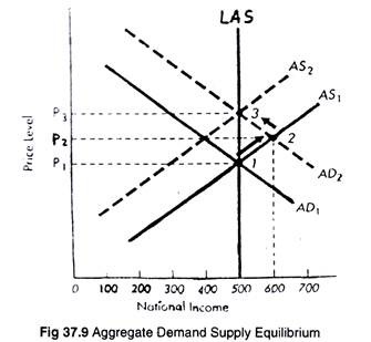
After studying the AD and AS curves separately we may now put both the curves in the same diagram to determine the equilibrium level of price and na­tional income. Fig. 37.9 shows such an equilibrium. Initially equilibrium occur at point 1, at which the AD₁ and AS₁ curves intersect. Here the price level is P₁and national income is Rs. 500.

This is an ex­ample of short-run equilibrium of AD and AS. If now AD increases, and the AD curves shifts to AD₂, in the short run a new equilibrium is established at point 2, where AD₂ intersects AS₁. Now the price level rises to P₂, and the equilibrium level of national income also increases to Rs. 600.

Over time as wages and other resource prices rise in response to higher prices, aggregate supply falls, shifting AS₁ to AS₂. The economy finally reaches equilibrium at point B, as is indicated by the left­ward pointing arrow. This means that the price level now rises to P₃, with the equilibrium level of national income returning to its original level (Rs. 500).

Long-Run Equilibrium:

In the long run shifts of AD or AS curve will only lead to changes in the general price level, with no change in equilibrium output. Point 3 in Fig. 37.9, for example, shows a higher price level (P₃) but the same level of output (Rs. 500).

This is so because there is no relationship between prices and the equilibrium level of national income (output). Again this is due to the fact that the costs of resources get adjusted to changes in the level of prices.

As Boyes and Melvin have put it, “The initial shock to or change in the economy is an increase in aggregate demand. The change in aggregate expendi­ture—initially leads to higher output and higher prices. Over time, however, output falls back to its original value while prices continue to rise. This is a major difference between the aggregate expenditure and income model of the economy and the aggregate demand and supply model. When prices are fixed, as they are in the Keynesian model, an increase in ag­gregate expenditures increases national income by a multiple of the initial increase in expenditure.”

This means that in this flexible price model, an increase in aggregate expenditure increases national income only temporarily. Ultimately the model produces higher prices at the same level of national income.

However, we should not make the prediction that the level of output never changes. We have noted that the AS curve shifts as technology changes and new supplies of resources are obtained.

But in comparison to the fixed-price model, the output effect that is observed here due to charges in aggregate expenditures is totally a temporary phe­nomenon. The general price level eventually adjusts, and output returns to its potential (full-capacity) level.

Recap:

1. The equilibrium level of price and national in­come (output) is determined at the/point where the AD and AS curves intersect.

2. In the short-run, a shift in AD establishes a tem­porary equilibrium along the short-run AS cur­ve, with changes in both price level and national output.

3. In the long-run, when AS and AS curves shift, there are changes in the general price level with no change in equilibrium level of output or na­tional income.