General Equilibrium of Product and Money Market

General Equilibrium of Product and Money Market!

There can be several equilibrium pairs of Y and r for both money and product market. But there is single pair of Y and r which emerges from the intersection of IS and LM curves that ensures equilibrium in both money and product markets.

Equilibrium attained like this is also known as general equilibrium, since it establishes equilibrium in the money market, bonds market and the product market.

Adjustment towards equilibrium assumes two things:

1. Interest rate changes according to the position of demand for and supply of money,

2. Income level changes according to the position of demand for output.

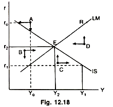
Edward Shapiro believes that in case of disequilibrium both the markets adjust simultaneously. Whereas, William H. Branson is of the opinion that money markets adjust much faster than the product market. The question how does an economy attain general equilibrium can be examined with the help of Fig. 12.18.

Point E shows general equilibrium. All the points left of LM curve take A, L & B indicate that at their respective levels of income, rates of interest are higher than the rates required to establish equilibrium in the money market. For instance, at A which has a pair of r₀ and Y₀, where r₀ is too high a rate of interest to establish equilibrium in the money market.

This is a situation of excess money supply over money demand. Rate of interest must fall to r₁ to bring equilibrium in the money market. But at r₁ (I + G) is so high that through multiplier income would start rising beyond Y₀. This rise in Y will increase the transaction demand for money which would be shifted from speculative demand for money raising the interest rate. This rise in r would reduce the private business investment, known as crowding out of investment, lowering the income from Y₁ level. Ultimately r₂, and Y₂ levels would settle and both the markets would be in equilibrium at E.

Similarly, at all points beyond IS curve output is more than the aggregate demand I + G. Output will adjust according to demand. Thus a change in output or income would change the transaction and speculative demand for money bringing thereby, a change in the rate of interest. These changes will continue till r₂ and Y₂ levels are reached establishing equilibrium in money, bond and product market.

Naturally, a shift in either IS or LM curve will bring a change in general equilibrium condition and will settle where the new IS and LM curves are intersecting each other.

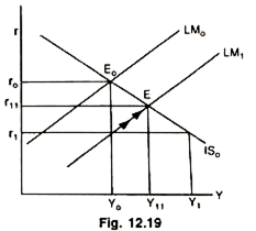
Initially the economy is in general equilibrium at E₀ where LM₀ and IS₀ intersect each other establishing r₀K₀ pair of interest rate and income level. Increase in money supply shifts the LM curve to LM₁ establishing r₁ rate of interest at K₀. As r falls to r₁ investment will increase and raise the multiplied income to Y₁ in a static model where all changes are instant.

Increased Y will demand more money for transaction purposes which shall flow out of speculative balances, r will rise and it will result into crowding out of private investment. Ultimately, E₁ point, the point of general equilibrium will be attained establishing r₁₁ and Y₁₁ levels or r and Y.

The IS and LM Elasticities and Monetary—Fiscal Policies:

We have seen the general characteristics of the IS and LM model called the general equilibrium model. It is not possible to carry on the analysis without taking into consideration the elasticities of IS and LM functions. For example, it will be seen, that it is possible that an expansionary fiscal policy may raise the interest rate without raising income level or may raise income level without raising interest rate.

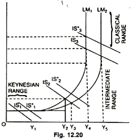
Similarly, an expansionary monetary policy may lower interest rate without changing income or it may change neither income nor rate of interest. The elasticities of IS and LM curves in different ranges are shown in the adjacent figure. In this figure the perfectly elastic portion of LM curve is called the ‘Keynesian range: the perfectly inelastic portion is called the ‘classical range’ and the portion in between is called the ‘intermediate range’.

In the Keynesian range of the figure, there is the famous ‘liquidity trap’ at which speculative demand for money may become perfectly elastic because wealth holders feel rate of interest will fall or cannot fall any more to a lower level. On the other extreme, at some very high rate of interest the speculative demand for money may become perfectly inelastic because wealth holders feel that rate of interest will rise no further—it is called the ‘Classical Range’ of the LM function.

Monetary policy means Central Bank’s control over the money supply. Fiscal policy means the government’s control over public spending and tax collection. The IS—LM framework provides a basis for comparing the effects of two types of policies on the income level and interest rate and for comparing the conditions under which each types of policy will be effective or ineffective.

1. Keynes treats Investment curve to be relatively interest-inelastic, therefore, it resulted into more dependence on fiscal policy. Price level is assumed to given in the entire treatment.

The Keynesian Range:

The Keynesian range is denoted by OY₁ income and or₁ rate of interest, i.e., y₁r₁. An increase in money supply shifts the LM curve to the right, from LM₁ to LM₂—which means that for each possible level of income M^s = M^d, only at a lower rates of interest. It is not true in the ‘liquidity trap’ range. Hence, the rate of interest has already fallen to the lowest possible minimum level on.

Hence, any expansion in money supply cannot cause the rate of interest to fall below the rate given by the trap, i.e., or₁. If follows that in the Keynesian range, monetary policy is ineffective to raise the income level. It was this belief in the existence of liquidity trap in the Keynesian range in the early 1930s that led Keynes to his unorthodox fiscal policy prescriptions.

Since the government cannot raise the income level through monetary policy, whatever the government is to do through monetary—fiscal policy—it must then, do through fiscal policy alone. Fiscal measures, such as, increased spending, tax reductions, that may shift the IS curve from IS₁to IS’₁ became the order of the day. Hence, monetary policy was relegated to the background and fiscal policy became prominent. The liquidity trap is an extreme case that could occur only during a deep depression. A prosperous economy and a liquidity trap do not go hand in hand.

The Classical Range:

In the classical range (Y₄r₄), equilibrium is defined by the intersection of IS₃, and LM₁. There is some increase in money supply which shifts LM₁ curve to LM₂—it means an increase of income from Y₄ to Y₅ and a fall in the rate of interest from r₄ to r₃. In the classical range the rate of interest is so high (r₄) that the demand for speculative balances is almost nil; money is held for transactions purposes only. A fall in the rate of interest from r₄ to r₃ will encourage investment and produce a new equilibrium level of income. In this range, the result follows the simple quantity theory of money as a theory of aggregate demand. Y rises proportionately with the increase in M. In contrast to the Keynesian range, in which the monetary policy a completely ineffective, in the classical range, it appears to be completely effective—whereas the fiscal policy is quite ineffective. An upward shift in the IS curve from IS₃, to IS’₃ will raise only the interest rate, from r₄ to r₅; the income level being unchanged at Y₄. In the classical range, an increase in income is possible only with an increase in money supply.

The Intermediate Range:

Y₂r₂ equilibrium shows the intermediate range—as defined by the intersection of IS₂ and LM₁ curve. Here, when there is some increase in money supply, it shifts the LM₁ curve to LM₂. In the Keynesian range, the increase in” M left both Y and r unchanged. In this range an increase in M is absorbed partially in speculative balances and partially in transactions balances. The level of income rises somewhat but by an amount less than that which would require the full increase in M for transactions purposes.

Thus, in the intermediate range monetary policy is effective to some degree but not with complete effectiveness it has in the classical range. In general, the closer the equilibrium intersection is to the classical range, the more effective monetary policy becomes, and the closer the intersection is to the Keynesian range, the less effective it becomes.

Within this range, fiscal policy is also effective to some extent. Fiscal measures that shift the IS function from IS₂ to IS₂, for example, will raise the level of income and the rate of interest to the new equilibrium at the intersection of IS₂ and LM₁, we assume a fixed money supply described by LM₁; so the increased expenditure is being financed by borrowing from public or it is deficit- financed increase in government spending.

Thus, fiscal policy also has some effectiveness in the intermediate range but it will be more effective, the closer the equilibrium is to the Keynesian range and less effective the closer the equilibrium is to the classical range. Although both monetary and fiscal policies have varying degrees of effectiveness in the intermediate range, the relative effectiveness of each depends in large part on the elasticity of the IS function. If the IS function is inelastic, monetary policy can do very little to raise income level, even in the intermediate range, fiscal policy alone is effective in such a situation.

Keynes maintained that the investment demand schedule is interest-inelastic and therefore IS schedule must also be inelastic and fiscal policy alone which is very effective in Keynesian range, would be almost as effective in the intermediate range. That was the 1’eason, why he gave more importance to fiscal policy.

It may, however, be noted that though the general equilibrium model provides a determinate solution determining the equilibrium level of income and the rate of interest simultaneously, yet the model operates under certain limitations as pointed out by D.C. Rowan’ like the model being static, assumes a given price level does not take into account international trade and the complete working of the monetary system. Despite its limitations, the IS—LM general equilibrium model is a good tool of analysis.