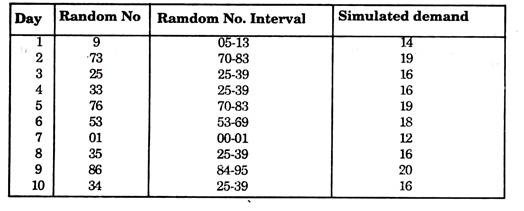
Read this essay to learn about the eight main techniques used for forecasting the demand for products. The techniques are:- 1. Opinion or Judgmental Forecasts 2. Consumer’s Opinion Surveys 3. Extensions of Past History 4. Association with Other Events 5. Market Research Method 6. Exponential Smoothing Method 7. Method of Simulation 8. Markovian Process Method.
Essay # 1. Opinion or Judgmental Forecasts:
It is one of the most widely used and influential forecasting techniques where the opinions and intuition of management is utilized. The process brings together in an organized manner, personal judgments about the process being analysed.
Main reliance is on human judgment. In this method, the executive uses his own anticipation and what he hears from other. Outside experts are also consulted and the other executive heads are also required to give their opinion- in the matter, Salesmen are to provide information about customer’s attitude and preferences and the activities of competitors.
Thus all possible information from the opinions of various persons is combined together to change the subjective opinions in to quantitative forecasts.
ADVERTISEMENTS:
No doubt experts and experienced managers can be useful as guides and serve as reliable source of information, but one has to make his own decision from all the opinions. Thus in this method broad guess is made by the executive in charge of a business.
There are many advantages and disadvantages of opinion technique of forecasting:
Advantages:
(i) Simple and easy to understand.
ADVERTISEMENTS:
(ii) No specialized skill is required i.e. less mathematical sophistication.
(iii) Low cost.
(iv) Is based on the information or opinion of the persons who are directly involved in the system.
(v) Can be used when satisfactory data is not available.
ADVERTISEMENTS:
Disadvantages:
(i) Opinions and intuitions are highly subjective.
(ii) Personal estimates are likely to be biased.
(iii) Time required to take the decision may be more.
(iv) Results can be easily distorted.
(v) Lacks scientific validity.
(vi) Is not based on valid facts.
(vii) The method is not useful for long term planning.
The method can be useful for many new products or new service estimators where sufficient past experience is not available.
Essay # 2. Consumer’s Opinion Surveys:
ADVERTISEMENTS:
This is a straightforward method to make short-term sales forecasts. The investigators and their preferences and attitude to words the product as well as future requirements are ascertained directly contact the consumers. This information is then used to project the sales for future.
This method is appropriate when the consumers of the product are industrial producers purchasing the item in large quantities. This method is not suitable to make long term forecasts for the consumer or household products which are affected by change of attitudes and fashions.
Essay # 3. Extensions of Past History:
Basically all statistical approaches of forecasting project historical information into the future. These are based on assumption that one can make useful predictions by studying the past behaviour i.e., the factors which where responsible in the past will also be operative to the same extent in future.
Some companies have detailed sales record item wise as well as territory wise. These sales records can be utilized to make useful predictions. The information should be complete with respect to events, policies, and quality of the product etc. from period to period.
ADVERTISEMENTS:
Such information in general is known as Time series data.
The time series for any phenomenon is composed of three components:
(i) Trend:
Trend exhibits the general tendency of the data and is downward, depending on the behavior.
ADVERTISEMENTS:
(ii) Seasonal Variation:
Seasonal components give information about the seasonal or cyclical behavior of the phenomenon. These are repetitive in nature.
(iii) Random Fluctuations:
Random variations are chance variations and cannot be used for forecasting.
Mostly trend is used for forecasting in practice. There are many methods to determine trend.
Some of the methods are:
ADVERTISEMENTS:
(a) Graphical method.
(b) Least square method.
(c) Moving average method.
(a) Graphical Method:
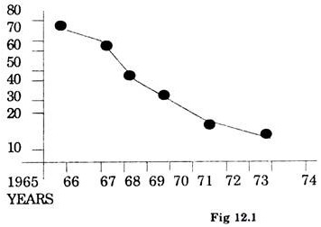
In this method the period is taken on x- axis and the corresponding sales values on Y-axis and the points are plotted for given data on graph paper. Then a free hand curve passing through most of the plotted points is drawn. This curve can be used to forecast the values for future.
The methods are explained by the following example.
ADVERTISEMENTS:
Example. 1:
The demand for a product is continually diminishing.
Estimate the demand for 1974 with the help of following information:
Solution:
Plot a graph for the given data to find the demand for 1974 see fig. 12.1. From thee graph for the given data to find the demand for 1974 comes out to be approximately 20, 000 units.
ADVERTISEMENTS:
It is an approximate method as the curve mainly depends on the choice of the scale for the graph and the individual who draws the free hand curve.
(b) Least Square Method:
This is one of the best methods to determine trend. In most cases, we try to fit a straight line to the given data. The line is known as ‘Line of best fit’ as we try to minimise the sum of the squares of deviation between the observed and the fitted values of the data. The basic assumption here is that the relationship between the various factors remains unchanged in future period also.
Let Y denote the demand and X the period for a certain commodity. Then the linear relationship between Y and X is given by
Y = a + bx ….(12.1)
ADVERTISEMENTS:
The nature of the relationship is determined by the values of a and b. The values of a and b can be estimated with the help of the past information about Y and X, if x and y denote the deviations of X and Y from their respective means, then the least square estimates of a and b are given by
â = Σy/n
b̂ = Σxy/Σx2 …..(12.2)
Where n is the number of observations.
The calculation of ∑y, ∑xy and ∑x2 can be done with the help of given data on Y and X and using the following steps:
Steps in least square calculations:
(i) Find means of Y and X say My and Mx
(ii) Find deviations of X and Y from their means i.e.
x = X – Mx and y = Y – My
(iii) Multiply corresponding deviations of X and Y and find their sum to get ∑xy.
(iv) Find the square of deviations for X and take the sum to get ∑x2.
(v) Use (12.2) to estimate the values of â and b̂
The method is illustrated by the following examples.
Example2:
Find the trend by least square method for data in Example 1, and forecast the demand for the year 1974.
Solution:
Let the trend line be given by
Y = a + bX,
where X denotes Time and Y the corresponding demand.
Then by least squared method
â = Σy/n
b̂ = Σxy/Σx2
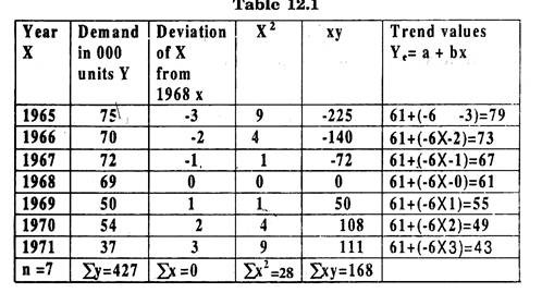
The calculations can be done in the tabular form 12.1
Here x = X. (Some value of X in middle)
Now Y = a + bX
and if we take deviations of X from its mean, then
Y = b̂ + ax
where
Form table (12.1), ∑Y = 427, n = 7,CY = 427, n = 7, ∑x2 = 28 and ∑xy = -168.
Hence â = 427/7 = 61
b̂ = ∑xy/∑x2 = – 168/28 = – 6
So the line of best fit is
Y = 61 – 6x, but x = X – MX
= 61 – 6 (X x MX), MX = ∑X/n = 1968
= 61 – 6(X – 1968)
For X = 1974
Y = 61 – 6(1974 – 1968)
= 61 – 36 = 25000 units.
Example 3:
The product group sales and product M sales are given below:
Fit a linear trend and forecast the sales (both product group and product M) for the year 1976.
Solution:
Let years be denoted by X and product group sales by Y. Then linear trend of year X is given by
Y = a + bX
The unknown constants ‘a’ and ‘b’ can be estimated by least square method. The calculation can be done in the following tabular form.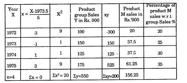
b̂ = ∑xy/∑x2 = 200,000/20 = 10,000
For x = 1976, forecast of Group Sales will be
Hence the linear trend is
Y = 1,37,500 + 10,000 [(X – 1973.5)/.5]
= 1.37,500 + 10,000 (5)
= 1,87,500.
Forecast for Product ‘M’ Sales in 1976:
It can be observed from the percentages of Product ‘M’ sales w.r.t Group sales, that every year there is and increase of 5% from the percentage of the preceding year. Hence the percentage of Product ‘M’ sales in 1976 will be 40% of group sales in 1976.
i.e. 40 x 1,87,500/100 = R.s. 75,000
Note:
If the pattern of change in percentage is not clear then one can take the average of the percentage of all the four years and forecast the sale for product ‘M’ e.g., in this case the average percentage is (20 + 25 + 30 + 35)/4 = 27.5 and 27.5 % of 1, 87,500 is Rs. 51, 562, 50 is the sales of product M in 1976.
An advantage of least squares method:
(i) There is no need to conduct any sample survey, as only past information about sales is required.
(ii) Method is simple and easy to understand.
(iii) Under normal situation the method is likely to give reliable and accurate results.
Disadvantages of least squares method:
(i) The method is based on some mathematical formulae, which may not be understood by common man.
(ii) The assumption that other things remaining constant may not hold good in practice.
(c) Method of Moving Averages:
This method can be used to determine the trend values for given data without going into complex mathematical calculations. The calculations are based on some predetermined period in weeks, months, years etc. The period depends on the nature of characteristics in the time series and can be determined by plotting the observations on graph paper.
A moving average is an average of some fixed or pre-determined number of observations (give by the period) which moves through the series by dropping the top item of the previous averaged group and adding the next item below in each successive average.
The calculation depends upon the period to be odd or even.
In the case of odd order periods (3, 5, 7…) the average of the observations is calculated for the given period and the calculated value is written in front of central value of the period e.g. for a period of 5 years, the average of the values of five years is calculated and is recorded against the third year. Thus in case of five yearly moving averages, first two years and last two years of the data will not have any average value.
If period of observations is even four years, then the average of the four yearly observations is written between second and 3rd year values. After this centering is done by finding the average of the paired values. The method is illustrated by solving example.
The even order periods creates the problem of centering between the periods. Due to this generally odd order periods are preferred. The calculated values of the moving averages became the basis for determining the expected future sales.
If the underlying demand pattern is stationary i.e. at a constant mean demand level except, of course, for the superimposed random fluctuations or noise, the moving averages method provides a simple and good estimate. In this method equal weight age is assigned to all the periods chosen for averaging.
The moving average method for forecasting suffers from the following defects:
(i) Records of the demand data have to be retained over a fairly long period.
(ii) If demand series depicts trend as against the stationary level the moving average method would provide forecasts that lags the original series.
Example 4:
The following are the annual sales in thousands of a product during the period 1965-1975.
Find the trend of the sales using (i) 3 yearly moving averages (ii) four yearly moving averages and forecast the value for the year 1977.
Solution:
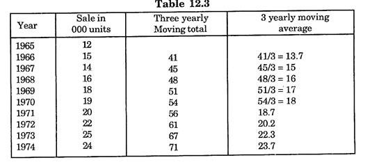
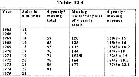
The trend values can be calculated in the following tabular form:
(i) 3 Yearly Period:
e.g 41= value of 1965 + value of 1966 + 1967 = 12 + 15 + 14 = 41 written at the central period 1966 of the years 1965, 66 and 67,
(i) Four Yearly Moving Averages:
*57 = value of 1965 + Value of 1966 + Value of 1967 + Value of 1968
= 12 + 15 + 14 + 16
= 57 written between 1966 and 1967.
**120 = 57 + 63,128 = 16 + 65…………. written in the center of 1966, 1967,
1968 i.e. 1968 and so on.
***120 is the total of 8 years. So average is calculated by dividing 120 from 8.
To avoid the problem of centering, generally odd periods are taken for moving averages computations.
Forecast for the Year 1977:
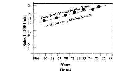
The trend values from the table 12.3 and 12.4 can be plotted on graph paper to estimate the value 1977 see fig. 12.2.
Sale of 1977 from three yearly moving averages Trend is 25000 units.
Trend value for 3 yearly and 4 yearly moving averages is almost same.
Merits of Moving average method:
(i) The method is simple and easy to apply in practice.
(ii) It is based on mathematical calculations.
(iii) More accurate than graphical method.
Demerits:
(i) Choice of period of moving average is difficult.
(ii) Cannot be applied if some observations are missing.
(iii) Some trend values for the periods in the beginning as well as in the end cannot be determined.
(iv) When the period of the moving average coincides with the periodicity in the data, if any, then the trend values may not be representative.
Essay # 4. Association with other Events:
The sale of any commodity does not depend on time only but there are some other economic factors viz. change in population, income, size of the families, tastes of the consumer, environment etc. Which can affect the demand of a product. The nature of relationship between these factors and the sales can be used to forecast future sales.
Assuming the relationship to be linear, the regression of Y on X can be defined as
Y = a + bX, a and b can be estimated by least square methods
where Y̅ and X̅ are the means of Y and X, σy and σX are their respective standard deviations, r is the simple correlation coefficient between X and Y. The two relationships can be used to forecast the value of Y for given X.
The following are the various steps in the methods:
(i) Verify whether there exists any relation between the demand of the product and the corresponding economic indicator or not.
(ii) If the relationship exists, then assuming the relationship to be linear, estimate the equation Y = a + bX by least square method or find the regression equation Y on X.
(iii) It is not necessary that the same relationship as in past may hold good in future also. Thus there is a need of proper judgement and consideration of new factors as well.
The technique appears to be easy and simple to apply in practice. But it is difficult to select the appropriate economic indicator, which can affect the sales. The method requires specialized skill and in some situations there may be a necessity to change the economic indicator of past data due to changes in fashion, nature and customs.
The method is illustrated by the following example:
Example 5:
The following is the demand of room coolers in five towns during the year 1980.
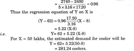
Fit a regression line of Y on X and estimate the demand of coolers for a city of population 50 lakhs.
Solution:
The regression equation is given by:
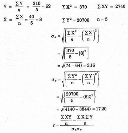
The following calculations can be made from the given data
Essay # 5. Market Research Method:
Big business houses generally use this method. A separate marketing research cell is established in the organization, which collects the required information both from internal and external sources for sales forecasting. Field surveys are also conducted to get direct information from the potential consumers and retailers.
The collected information is processed and analyzed by the department of the enterprise using statistical techniques like time series analysis, Correlation analysis etc.
The following are the advantages and disadvantages of this method:
Advantages:
(i) Helps in quick decision making by supplying regular and systematic information.
(ii) The accuracy of the results can be tested by statistical methods.
(iii) Detailed study of the problem is possible.
Disadvantages:
i. Method is expensive and can be afforded by big organizations only.
ii. The results should be regularly reviewed and adjusted to changing conditions.
Essay # 6. Exponential Smoothing Method:
This method is an improvement over moving average method of forecasting. It tries to overcome the limitations of moving averages and eliminates the necessity of keeping extensive records of past data. It also tries to screen out the irregularities in the demand pattern. The method allows for trend and takes into consideration the short-term fluctuation in the determination of the forecast.
Exponential smoothing is also a weightage average of the observations. Here the most recent observation is assigned the highest weight age and it decreases in geometric progression as we move towards the older observation. It is considered to be more realistic than moving average where past observations carries just as much weight as latest.
In fact the later figures will tend to reflect the more up to date average of the series and it would be better if they could be given more weight than the earlier figures in the calculation. Exponential Weighting is, however, a neater and easier method of achieving a progressive form of weighting.
Here all one does, each period is to suitably weight and then add together the current figure and the previous period’s moving average.
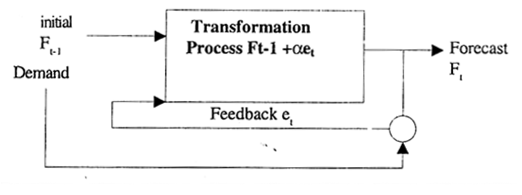
The fundamental concept of exponential smoothing method is that:
New estimate = old estimate of least actual demand + α (Latest actual demand – old estimate of least actual demand)
Ft = α Dt + (1 – α)Ft -1 = F t – 1 + α et
where Ft is the Forecast at time t
Dt is the actual demand at time t
Ft-1 is the forecast at time (t-1)
α is the smoothing coefficient, et = (Dt– Ft-1,)
The computational procedure is summarized below:
(i) Find error by subtracting the recent average from the least incoming observation.
(ii) Multiply error et by α.This is the correction to be applied to the past average.
(iii) Add correction (α et) to the past average, Ft-1. This gives new average Ft as the forecast for the next period.
The performance of this method depends on the value of the smoothing co-efficient α and the initial forecast Ft-1
The selection of a value for a gives the selector a measure of control over the degree of smoothing induced in the series and its choice depends on how much weight is desired to be given to later periods relative to earlier periods. A low value of α gives more weightage to the past figures and less consideration to incoming observation.
Low values of the smoothing coefficient are used where the series is rather stable and high values where the series is fluctuating. Thus the size of α will depend on the speed with which one wishes against the risk of making forecasts errors. The value of α lies between 0 and 1.
Although a high smoothing constant keeps the average more closely aligned to the actual figures but it don not necessarily contributed to better forecasts and is unduly influenced by random variations. If cyclical are fluctuation predominant in forecast then one should take low value of α and in case long term fluctuations are more dominant then take high value of α.
Two main factors should be considered in selection of α:
(i) Distribution of random errors.
(ii) Costs associated with forecasting errors.
In practice α is generally chosen between 0.1 and 0.3.
The choice of initial forecast Ft -1 is either based on subjective estimates or as simple arithmetic average of the past few periods. Here one may have some inaccuracy in earlier forecasts but may take quite a few periods for the forecasting model to wash out.
Exponential Smoothing Forecasting System
Exponential smoothing provides a convenient, systematic and recursive method for revising the forecast for the next period whenever discrepancy exists between the previously forecast demand for current period and the actual demand for current period and the actual demand for current period. The amount of adjustment is determined by the selected smoothing coefficient- the greater the coefficient the greater is the adjustment and vice-versa.
Box-Jenkins Method:
This forecasting approach has been borrowed from the control theory. In a control system, there is a target, which has to be tracked where the target itself is moving or changing its value or position. The control mechanism measures the difference between the target and actual output.
Analogous to the target is the demand in the forecasting system that is sought to be tracked by the forecasting. Any error is used along with its derivatives and integrals for improving the forecast for the next period and so on.
The basic equation is New Forecast = Old forecast + the direct term: A (error in old forecast) + time derivative term: B (change in error between last time and time immediately before + the integral term: C (Sum of the errors so far)
Essay # 7. Method of Simulation:
There are many problems experienced in everyday life, which cannot be satisfactorily represented by some mathematical model or sometimes the model becomes so much complicated that its solution by analytical method is not possible. In such situation Simulation or Monte- Carlo methods are found to be useful.
The name monte-carlo has been generally used for a method where distributions functions are determined with the help of random numbers. Pioneers in the field are Von Neumann, Ultam and Fermi.
A simulation model is an image of reality, which allows the solution of a problem by trial and error approach. Dr. A.S. Householder defines Monte Carlo techniques as the device for studying an artificial stochastic model of a physical or mathematical process. Simulation methods are combinations of probability and sampling methods, providing solutions to complicated problems.
It is particularly useful in situation where it is not possible to gain practical experience because one has to deal a problem, which has not yet arisen.
A good simulation model should be:
(i) Accurate,
(ii) Acceptable to the problem and
(iii) Quick to generate.
General simulation method is based on the selection method is based on the selection of random numbers tables and these numbers are considered to be the probabilities of desired characteristic understudy drawn from the parent population.
The random numbers are recorded from the random number tables in a systematic way i.e. once recording of the numbers are to be recorded from the chosen pointed till required observations are drawn. It is assumed that the characteristics observations in the sample as well as the production are same.
Following are the steps in Simulation method of forecasting:
(i) Past behaviour of the system is determined by conducting some preliminary survey. Generally this is done with the past data available in records.
(ii) Some appropriate model is selected for the system with the help of sample observations obtained in step (i).
(iii) The model in step (ii) is used to determine the probability distribution of the characteristics under study. The probability distribution can be easily changed into cumulative distribution function.
(iv) Random numbers are chosen from random number tables and are then used to find the sequence of values of the variable of interest.
(v) Some standard mathematical function is fitted to the values obtained in step (iv).
The application of simulation method for demand forecasting is explained with the help of the following example:
Examples 6:
A fish market owner wishes to generate a series of Friday’s demand for mullet. It has been determined from past demand data that the demand is normally distributed with mean values 175 kg.
And standard deviation 25 kg.
Solution:
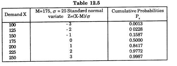
It is known that 99.7% of the observations in standard normal population lies in M + 3σ limits, where M and σ are respectively the mean and standard deviation of the normal population. Here also demand of mullet is given to be normally distributed with mean 175 and standard deviation 25. Thus 99.7% of the demand will be between 175 + 3 (25) i.e. 100 and 250 limits.
So we take some values between 100 to 250. Convert these into standard normal variate by the formula
Z = X – M/σ
and then read the cumulative probabilities from standard normal tables. The calculations can be recorded in the tabular form. (Table 12.5)
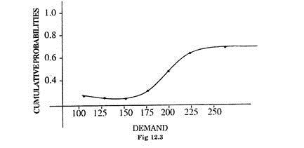
Table 12.5 provides the fitted distribution of demand for meat, These values are then plotted on the graph paper taking demand X on X-axis and the corresponding probabilities on Y-axis to get the graph in fig. 12.3.
Now to generate the Friday demand, random numbers are recorded from random number tables. Let the numbers be 22, 36, and 84… The demand for each number can be read from the graph in fig. 12.3. e.g. the number 84 in term of probabilities can be taken as 0.84 and the demand for p(x) = 0.84 from graph (12.3) is approximately equal to 200 kg. Similarly demand for other random numbers can be estimated.
Example 7:
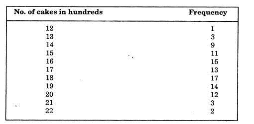
A bakery has collected the following data on weekend demands for cakes.
Simulate requirements for 10 weekends.
Solution:
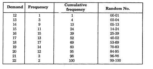
Here first of all the probability distribution from the given data is determined by preparing the following table:
Now for simulating the demand for 10 weekends read the 10 random numbers from the random number tables.
Essay # 8. Markovian Process Method:
Any stochastic process, which develops with time according to some law of probability, is known as Markov process. At every point of time the process is exactly in one of its possible outcomes at some point of time.
Markov process, in characterised by its transitional matrix which is a set of initial and transitional probabilities. The transitional matrix gives the step-by-step transitional probabilities of a Markov process.
The matrix has following properties:
(i) Each element of the matrix should be some probability.
(ii) The sum of the elements of each row in the matrix should be equal to one i.e. the process at some point of time should be in any one of the states.
The concept can be explained with the help to the following examples:
Example 8:
Three manufactures A.B and C are competing with each other.
The following matrix gives the transitional probabilities that customer will move from one manufacture to the other in any month.
Interpret the matrix in terms of (a) retention and loss (b) retention and gain.
Solution:
Each element of the matrix has a value between 0 and 1 the sum of elements in each row is exactly one? Thus the given matrix is transition matrix.
Each manufacturer can use each row of the matrix to interpret the monthly retention and loss.
Row I:
It is observed that A retains 70% of its customers but looses 10% to B and 20% to C.
Row II:
B retains 80% of its customer but looses 10% to A and 10% to C.
Row III:
C retains 70% of its customer but looses 20% to A and 10% to B.
Now suppose in the beginning there were 1000 customers with A, 2000 with B and 3000 with C, what will be the number of customers with each one of them after one month?
Using the above transition matrix, the following will be the number of customers with each manufacturer:
Thus A gains 500 customers, B have the same number of customers, Whereas C looses 500 customers.
Example 9:
Suppose an experiment is conducted and it is found that system is stable and is of Markovian Type. The market system is divided in to two categories at any time ‘t’ Non-customer and customers. It is observed that over some specified interval of time, 40% of the Non- customers change to customer in the market whereas 30% of the customers leave the market. The information is collected for 200 people.
The information can be expressed in the following matrix form:
These figures can be converted into transitional probabilities by dividing each row from 100. So the matrix of transitional probabilities will be
Let there be 10,000 people at time t = 1, then from the above transitional matrix we can find the Non-customers and customers at time t2 using the relations.
Non customers at time t2 i.e. NCt2 = 0.6 NCt1+ 0.3 Ct1
Customer at time t2 i.e. NCt2 = 0.4 NCt1 + 0.7 Ct1
In the beginning at time t = 1 all people are Non-Customers. Thus at t = 1, NCt1= 10,000 and Ct1 = 0.
Hence NCt2 = 0.6 (10,000) + 0.3 (0) = 6000
Ct2 = 0.4 (10,000) + 0.7 (0) = 4000
Assuming the behaviour of the customers and Non-customers and Non-customers to be uniform at different time periods, we can calculate the Non-customers and customers and different time periods, using the information of the preceding period e.g.
NCt3 = 0.6 NCt2 + 0.3Ct2
Ct3 = 0.4 NCt2 + 0.7Ct2
NCt3 = 0.6 (6000) + 0.3 (4000) = 4800
Ct3 = 0.4 (6000) + 0.7 (4000) = 5200
Similarly,
NCt4 = 0.6 (4800) + 0.3 (5200) = 4440
Ct4 = 0.4 (4800) + 0.7 (5200) = 5560
The process is continued till there is very little difference between the values of Non-customers or customers at two successive periods of time.

