Essay on Economic Statics and Dynamics

In this essay we will discuss about Economic Statics. After reading this essay you will learn about: 1. Meaning of Economic Statics 2. Meaning of Economic Dynamics 3. Comparative Statics 4. Significance of Economic Dynamics 5. Stationary State of Economics.

Contents:

1. Essay on the Meaning of Economic Statics
2. Essay on the Meaning of Economic Dynamics
3. Essay on Comparative Statics
4. Essay on the Significance of Economic Dynamics
5. Essay on Stationary State of Economics

---

Essay # 1. Meaning of Economic Statics:

The word ‘statics’ is derived from the Greek word statike which means bringing to a standstill. In physics, it means a state of rest where there is no movement. In economics, it implies a state characterised by movement at a particular level without any change.

It is a state, according to Clark, where five kinds of changes are conspicuous by their absence. The size of the population, the supply of capital, methods of production, and forms of business organisation and wants of the people remain constant, but the economy continues to work at a steady pace.

“It is to this active but unchanging process” writes Marshall, “that the expression static economics should be applied.” Static economy is thus a timeless economy where no changes occur and it is necessarily in equilibrium.

Indices are adjusted instantaneously:

Current demand, output and prices of goods and services.

As pointed out by Samuelson:

“Economic statics concerns itself with the simultaneous and instantaneous or timeless determination of economic variables by mutually interdependent relations.” There is neither past nor future in the static state.

Hence, there is no element of uncertainty in it. Kuznets, therefore, believes that “static economics deals with relations and processes on the assumption of uniformity and persistence of either the absolute or relative economic quantities involved.”

In addition, such assumptions as the existence of perfect competition, perfect knowledge, perfect foresight and perfect mobility are considered essential for the working of a static analysis. But Harrod does not consider these assumptions essentially relevant to static analysis.

Joan Robinson’s Imperfect Competition and Chamberlin’s Monopolistic Competition are exercises in economic statics. Economists explain static analysis in terms of micro- and macro-static equilibrium models.

Micro-Statics:

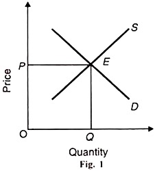
An economic model refers to relationships among different economic variables in which one variable appears in more than one relationship. In the micro-static models, supply and demand relationships determine prices at a point of time which are also constant through time.

The given demand and supply functions are:

D = (P)…. (1)

S = f (P)…. (2)

From (1) and (2) D = S…. (3)

where D is amount demanded of some commodity, S is amount supplied of that commodity and P is its price. This micro-static relationship is illustrated in Figure 1. D and S are the demand and supply curves respectively. They intersect at point E where amounts demanded and supplied equal OQ at the price OP.

In the absence of change in demand and supply conditions, this equilibrium position will apply not only to the present (point of time) but also to the future (through time). Hicks’ definition of economic statics that we use the term economic statics for those parts of economic theory where we do not trouble about dating fits in this explanation.

In his book Capital and Growth, Hicks defines economic statics more clearly as “one in which certain key variables (the quantities of commodities that are produced and consumed, and the prices at which they are exchanged) are unchanging.”

Macro-Statics:

Macro-static analysis explains the static equilibrium position of the economy.

This is best explained by Prof. Kurihara in these words:

“If the object is to show a ‘still picture’ of the economy as a whole, the macro­ static method is the appropriate technique. For this technique is one of investigating the relations between macro-variables in the final position of equilibrium without reference to the process of adjustment implicit in that final position.”

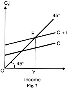
Such a final position of equilibrium may be shown by the equation Y= C + I where Y is the total income, С is the total consumption expenditure and I, the total investment expenditure.

It simply shows a timeless identity equation without any adjusting mechanism. In this static Keynesian model, the level of national income is determined by the interaction of aggregate supply function and the aggregate demand function.

In Figure 2, 45° line represents the aggregate supply function and C + I line, the aggregate demand function. 45° line and C + I curve intersect at point E. It is the point of effective demand which determines OF level of national income. Thus economic statics refers to a timeless economy.

It neither develops nor decays. It is like a snapshot photo from a ‘still’ camera which would be the same whether the previous and subsequent positions of the economy were subject to change or not.

---

Essay # 2. Meaning of Economic Dynamics:

Economic dynamics is the study of change, of acceleration or deceleration. According to Prof. Ackley, “Dynamics is concerned essentially with states of disequilibrium and with change.” It is the analysis of the process of change which continues through time or over time.

An economy may change through time in two ways: without changing its pattern and by changing its pattern. Economic dynamics relates to the latter type of change.

If there is a change in population, capital, techniques of production, forms of business organisation and tastes of the people—in any one or all of them—the economy will assume a different pattern, and the economic system will change its direction.

In the accompanying diagram, given initial values of the economy, it would have proceeded along the path AB, but suddenly at A the indices change the pattern, and the direction of the equilibrium changes towards C. Again, it would have preceded to D but at С the pattern and direction is changed to E. Thus, economic dynamics studies the path from one equilibrium position to another: from A to С and from С to E.

Hicks in his Value and Capital define economic dynamics “as that part of economic theory in which every quantity must be dated.” But Harrod does not agree with this when he says: “In dynamics dating is no more necessary than in statics.”

He, therefore, suggests that dynamics should concern itself with the analysis of “continuing changes generated by the special nature of a growing economy.” Thus, according to him, dynamic economics is concerned with “the necessary relations between the rates of growth of the different elements in a growing economy.”

He considers once-over changes to fall within the domain of economic statics. Such changes imply a shift from one position of equilibrium to the other. In terms of our diagram a shift from A to С and from С to E without traversing the path is static economics. Hicks accept this view of Harrod in his Trade Cycles.

Ragnar Frisch, however, regards economic dynamics not only a study of continuing changes but also of the process of change. According to him, it is a system in which “variables at different points of time are involved in an essential way.”

“This is essentially the characteristic of a dynamic theory—to explain how one situation grows out of the foregoing situation,” opines Frisch. Thus, the study of economic dynamics involves the discovery of functional relationships of economic variables at different points of time.

To conclude, economic dynamics is, concerned with time-lags, rates of change, and past and expected values of the variables. In a dynamic economy, data change and the economic system take time to adjust it accordingly. Dynamic analysis can be explained in terms of macro- and micro-dynamic models.

Macro-Dynamics:

According to Kurihara, “‘Macro-dynamics’ treats discrete movements or rates of change of macro variables.”

He further writes:

“This method separates the process of trial and error into a series of continuously changing reactions and indicates, step by step, what cause is and what effect is. It describes the changing universe as it is related to previous or subsequent adjustments, it analyses the discrete and continuous changes of aggregates, the sequence of cause-and-effect events arising from some initial disturbance and the time-paths of macro-variables and aggregative relationships. Thus, the macro-dynamic method enables one to see a ‘motion-picture’ of the functioning of the economy as a progressive whole.”

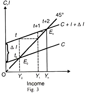
The macro-dynamic model is explained by Kurihara in terms of the Keynesian process of income propagation (the investment multiplier) where consumption is a function of the income of the preceding period,

i. e. С_t =f(Y) and investment is a function of time and of constant autonomous investment DI, i.e., I_t =f (DI). In Figure 3, C+I is the aggregate demand function and 45° line is the aggregate supply function.

If we begin in period t₀ where with an equilibrium level of income OY₀, investment is increased by DI, then in period t income rises by the amount of the increased investment (from t₀ to t). The increased investment is shown by the new aggregate demand function C+1+DI. But in period t, consumption lags behind, and is still equal to the income at E_o.

In period t+1 consumption rises and along with the new investment, it increases income still higher to OY₁ This process of income propagation will continue till the aggregate demand function C+I+DI intersects the aggregate supply function 45 line at E_n in the nth period, and the new equilibrium level is determined at OY_n. The curved steps t₀ to E_n show the macro­-dynamic equilibrium path.

The Cobweb Model (Micro Dynamics):

The cobweb model is used to explain the dynamics of demand, supply and price over long periods of time. There are many perishable agricultural commodities whose prices and outputs are determined over long periods and they show cyclical movements.

As prices move up and down in cycles, quantities produced also seem to move up and down in a counter-cyclical manner. Such cycles in commodity prices and outputs are explained in terms of the cobweb model, so called because the diagrams look like cobwebs.

Suppose the production process spreads over two periods: current and previous. Production in the current period is assumed to be determined by decisions made in the previous period. Thus the current output reflects a production decision made by the producer during the previous period.

This decision is in response to the price that he expects to rule during the current period when the crop is available for sale. But he expects that the price that would be established during the current period would equal the price during the previous period.

The cobweb model (or theorem) analyses the movements of prices and outputs when supply is wholly determined by prices in the previous period. In order to find out the conditions for converging, diverging or constant cycles, one has to look first at the slope of the demand curve and then of the supply curve.

If the slope of the demand curve is numerically smaller than the slope of the supply curve, the price will converge towards equilibrium conversely, if the slope of the demand curve is numerically greater than the slope of supply curve, the price will diverge from equilibrium. If the slop of the demand curve is numerically the same as that of the supply curve, the price will oscillate around its equilibrium value.

Its Assumptions:

The cobweb model is based on the following assumptions:

(1) The current year’s (t) supply depends upon the last (previous) year’s (t-1) decisions regarding output level. Hence current output is influenced by last year’s price, i.e. P (t-1).

(2) The current period or year is divided into sub-periods of a week or fortnight.

(3) The parameters determining the supply function have constant values over a series of periods.

(4) Current demand (D_t) for the commodity is a function of current price (P)-

(5) The price expected to rule in the current period is the actual price in the last year.

(6) The commodity under consideration is perishable and can be stored only for one year.

(7) Both supply and demand functions are linear.

The Model:

There are three types of cobwebs:

1. Convergent;

2. Diergent; and

3. Continuous,

They are explained as under:

1. Convergent Cobweb:

Under this formulation of the Cobweb Theorem, the supply function is S -S (t-1) and the demand function is D_t = D (P). The market equilibrium will be when the quantity supplied equals the quantity demanded: S_t = D_t in any market in which producers’ current supply is in response to the price during the last year, equilibrium can be established only through a series of adjustments that take place over several consecutive periods.

Let us take potato growers who produce only one crop a year. They decide about how many potatoes they will grow this year on the assumption that the price of potatoes this year will equal the price in the last year.

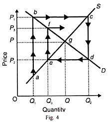
The market demand and supply curves for potatoes are represented by D and S curves respectively in Figure 4. The price in the last year was OP and the producers decide the equilibrium output OQ this year. But the potato crop is damaged due to a blight so that their current output is OQ₁ which is smaller than the equilibrium output OQ.

This leads to rise in the price to OP, in the current period. In the next period, the potato growers will produce OQ₂ quantity in response to the higher price OP₁ (= Qb). But this is more than the equilibrium quantity OQ which is needed in the market.

It will, therefore, lower the price to OP₂ (= Q₂d) and thus again lead to changes in the production plans of producers whereby they will reduce supply to OQ₃ in the third period. But this quantity is less than the equilibrium quantity OQ. Price will, therefore, rise to OP₃ (= Q_{3 f}) which, in turn, will encourage producers to produce OQ quantity. Ultimately, the equilibrium will be established at point g where D and S curves intersect.

The series of adjustments just described trace out a cobweb pattern a, b, c, d, e and f which converge towards the point of market equilibrium g when period-to-period changes in price and quantity have been reduced to zero. The cobweb is convergent. This is dynamic equilibrium with lagged adjustment.

2. Divergent Cobweb:

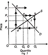
But there may be an unstable cobweb when price and quantity changes move away from the equilibrium position. This is illustrated in Figure 5. Suppose from the initial price-quantity equilibrium situation of OP and 00 there is a temporary disturbance that causes output to fall to OQ₁.

This raises the price to OP₁ (=Q₁a/ The increased price, in turn, raises output to OQ₂ which is more than the equilibrium output OQ. Consequently, the price falls to OP₂. But at this price the demand (OQ₂) exceeds the supply (OQ₃). As a result, the price shoots up to OP₃ (= Q₃e) and the adjustment of producers to this price leads farther away from the equilibrium.

This is an explosive situation and the equilibrium position is unstable. The cobweb is divergent.

3. Continuous Cobwebs:

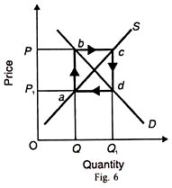
The cobweb may be of constant amplitude with perpetually oscillating prices and quantities, as shown in Figure 6. Suppose that the price in the current year is OP.

Thus the quantity to be supplied is going to be OQ₁ But in order to sell this output, the price that it will fetch in the next period will be OP₁ But at this price, the demand OQ₁ is more than the supply OQ which will raise again the price to OP(=Qb). In this way, prices and quantities will move in a circle with oscillations of constant amplitude around the equilibrium point e.,

Its Criticisms:

The analysis of the cobweb theorem is based upon very restrictive assumptions which make its applicability doubtful.

1. Not Realistic:

It is not realistic to assume that the demand and supply conditions remain unchanged over the previous and current periods so that the demand and supply curves do not change (or shift). In reality, they are bound to change with considerable divergences between the actual and expected prices. Suppose the price is so low that some producers incur heavy losses.

As a result, the number of sellers is reduced which changes the position of the supply curve. It is also possible that the expected price may be quite different from the estimated price. As a result, the cobweb may not develop properly on the basis of unchanged demand and supply curves. Thus demand, supply and price relations that lead to different cobwebs have little real applicability.

2. Output not Determined by Price:

The theory assumes that the output is determined by the price only in reality, the agricultural output in particular is determined by several other factors also, sue as weather, seeds’ fertilizer, technology etc.

3. Divergent Cobweb Impractical:

Critics hold that divergent cobweb is impossible. It is obvious from Fig. 4 that once the equilibrium is upset, the cobweb cycle goes on diverging for an indefinite period which leads to an explosive situation. It is Impossible.

4. Continuous Cobweb Impractical:

Critics point out that continuous cobweb is impractical because it cannot continue indefinitely. This is because producers incur more loss than profit from it. This is explained by Fig. 5. If a farmer producers OQ output, he receives total revenue OQbP whereas his total cost is OQaP₁ while the total cost is OQ₁cP.

Thus, he incurs P₁ dcP total loss. Hence, in the case of continuous cobweb cycle, the producers have to face alternative years of profit and loss, but losses always exceed profit. Therefore, ‘this cycle’ is impractical.

Its Implications:

1. The cobweb model is an oversimplification of the real price determination process. But it supplies new information to the market participants about the market behaviour which they can incorporate into their decisions.

2. The cobweb model is not merely an adjustment process of the market equilibrium but it also predicts unobservable events.

3. Its significance lies in the demand, supply and price behaviour of agricultural commodities. Expectations about future conditions have an important influence on current prices. If there are boom conditions in the country, the farmers expect higher prices of their crops and increase their supplies in the market.

But in the event of crop failures, the supplies of agricultural commodities will be reduced. In such a situation, the government may exempt farmers from agricultural taxes and even provide interest free loans to tide over the crisis.

On the contrary, a bumper crop may lower the prices of agricultural crops by increasing their supplies more than their demand. In such a situation, the government may give subsidies to farmers or procure agricultural products at minimum support prices from the farmers.

---

Essay # 3. Comparative Statistics:

Comparative statics is a method of economic analysis which was first used by a German economist, F. Oppenheimer, in 1916. Schumpeter described it as “an evolutionary process by a succession of static models.”

In the words of Schumpeter, “Whenever we deal with disturbances of a given state by trying to indicate the static relations obtaining before a given disturbance impinged upon the system and after it had time to work it out; this method of procedure is known as Comparative Statics.”

To be precise, comparative statics is the method of analysis in which different equilibrium situations are compared. The distinction between static, comparative static and dynamic situations is explained with the help of the accompanying figure.

If the economy is working at situation A where it is producing at a constant rate without any change in the variables, it is a static state which is functioning at a point of time. When the economy moves from the equilibrium point A to point В through time, it is economic dynamics which traces out the path of movement between the two equilibrium points.

Comparative statics, on the other hand, is related to once-over change from point A to point В in which we do not study the forces’ behind the movement between the two points. In other words, we simply compare the equilibrium position A with the equilibrium position B.

Thus comparative statics is not concerned with the transitional period but “involves the study of variations in equilibrium positions corresponding to specified changes in underlying data.”

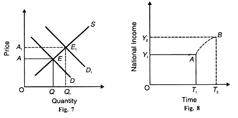
The Marshallian pricing process is based on the comparative static analysis where two equilibrium positions are compared, as shown in Figure 7. When the demand curve D intersects the supply curve S at point E, OB quantity of X is bought and sold at OA price.

With the upward shift in the demand curve from D to D₁ the new equilibrium is established at E₁. where OB₁ quantity of X is bought and sold at OA price. Here we do not study the causes or the process which led to the change from a lower to a higher equilibrium position. Rather, we say that the market sells and buys more quantity of A at a higher price OA₁ at point as compared with point E.

The Keynesian Employment, Income and Output analysis is also based on the theory of shifting equilibrium wherein he compares different equilibrium levels of income. According to Kurihara, Keynes made no attempt to show the process of transition from one position of equilibrium to another.

He simply used comparative static analysis. Figure 8 explains two different levels of income, OY₁ at OT₁ time and OY₂ at ОT₂, time. Income at OY₂ level is higher than at OY₁ level. This is comparative statics which compares two static levels of income as against dynamic economics which traces out the path AB, showing increase in income.

Importance of Comparative Statistics:

1. This method is praiseworthy for analysing the effects of causes which bring about disturbances.

2. It re-establishes stability in the process of change. If there are some changes in economic variables that lead to the process of continuing changes, it is not possible to tell when this process will end. Similarly, if once there is disturbance in the equilibrium which begins the continuous process of instability, it is not possible to tell definitely when the equilibrium situation will be restored.

In such a situation, comparative statics can show the direction of change by pointing towards some definite points of equilibrium. Thus this analysis provides certainty in an uncertain situation.

Limitations of Comparative Statistics:

But comparative statics is not without limitations:

1. Its scope is limited for it excludes many important economic problems. They are the problems of economic fluctuations and growth which can only be studied by the method of dynamic economics.

2. Comparative statics is unable to explain the process of change from one position of equilibrium to another. It “gives only a partial glimpse of the movements for we have only the two ‘still pictures’ to compare, whereas dynamics would give us a movie.”

3. We are not sure when the new equilibrium will be established because this method neglects the transitional period. This makes comparative statics an incomplete and unrealistic method of economic analysis.

Importance of Economic Statics:

Economic statics possesses both theoretical and practical importance.

(1) As a Teacher:

According to Zuethen, economic statics possesses an introductory pedagogic value. By assuming certain variables to be given and constant, it makes economic problems easy to comprehend. Economic statics provides an imaginary model of the economic phenomena in a state of rest which helps the student in understanding the consequences of certain changes.

For instance, the study of equilibrium price is valuable for understanding the behaviour of prices in an economy. In the static state, demand and supply are always in equilibrium. How do variations in demand and supply affect prices can only be understood when both demand and supply are in a state of equilibrium.

(2) For Investigation:

The traditional economists assumed static conditions for purposes of investigation. They studied the activities of individual firms, industries and consumers for the understanding of social phenomena. They made it applicable to the real world by giving it a little dynamic flavouring.

(3) To Study Comparative Statics:

Another advantage of static analysis is that it helps in comparing one position of equilibrium with that of another. This is comparative statics which is based on economic statics.

(4) To Solve Complex Problems:

Further, in economic statics one studies how an individual distributes his limited money income among various commodities in order to obtain maximum satisfaction; how a producer gets maximum profits by combining given productive resources in an optimal manner, how the prices of commodities and services are determined, and how is national income distributed.

The significance of static analysis lies in solving these complex problems.

(5) In Economic Principles:

Besides, a vast field of economic theory enumerated below is based on the study of economic statics.

The central core of the doctrine and principles relating to Robbins’ definition of economics essentially belong to economic statics. The case of free trade, the doctrine of international trade, Joan Robinson’s Economics of Imperfect Competition, Chamberlin’s Monopolistic Competition, and Hicks’ Value and Capital are all exercises in static analysis that have enriched economic theory.

(i) Uncertainty:

Since change and roundabout methods of production involve uncertainty and once­over change generates more uncertainty than a continuing change, Harrod “conceives Knight’s theory of profit to lie within the field of statics”. This is an attempt at solving one of the most bewildering problems of economics with the help of static analysis.

(ii) Expectations:

Expectations generally fall within the purview of economic dynamics. But the effects of a once-over change in expectations are handled by the technique of static economics. Concurring with this view of Roy Harrod, Hicks in his Trade Cycles regards Keynes’ General Theory as essentially static due to the presence of expectations in it.

(iii) Keynesian Theory:

With the exception of the concept of Positive Saving, all the variables in the Keynesian analysis are static in character. They are involuntary unemployment, liquidity preference, marginal efficiency of capital and marginal propensity to consume. His use of the principle of multiplier is also static. In explaining all these variables, Keynes shows once-over changes, the use of static analysis.

(iv) Trade Cycles:

Harrod believes that a trade cycle is experienced even by static states, when it represents regular and periodic fluctuations. The climatic, psychological and monetary theories of trade cycles before the Second World War were static in nature. Of late, Tinbergen, Kelecki, Frisch, Samuelson and Hicks have developed dynamic theories of the trade cycles by introducing time lags and the principle of acceleration.

Limitations of Economic Statics:

But static analysis has its weaknesses. It is away from reality. It assumes certain economic variables like population, tastes, techniques, etc. as given and constant. It excludes the influence of external forces and is thus related to a closed economy. All this makes static economics and the laws based on it unrealistic.

Further, economic statics disregards the influence of time. It is a timeless economy, whereas changes are continuously taking place in this world. Thus, economic statics is just a figment of imagination, an intellectual toy with which economists play. Such an analysis can, therefore, provide only a limited treatment for the study of economy problems.

---

Essay # 4. Significance of Economic Dynamics:

Economic dynamics possesses great significance in theory and practice.

1. It is Realistic:

The significance of economic dynamics lies in that it is a reality and not a fiction. It explains the causes and effects of changing economic phenomena and enables us to see a moving picture of the working of an economy how the economy develops in one period out of the preceding period.

2. Study of Stability of Equilibrium:

Further, it is a study not of equilibrium position but of changing equilibrium. Dynamic analysis studies the behaviour of the economic system in disequilibrium and traces the path of the forces that bring a new equilibrium position. Thus the important problem of the stability of equilibrium relates to dynamic analysis.

3. In the Study of the Problems of Classical Economics:

Some of the problems in classical economics also lend themselves to dynamic analysis. The Ricardian Theory of Distribution and the Malthusian Theory of Population are exercises in dynamic theory. Even the Marshallian distinction between short-run and long-run pricing pertains to dynamic analysis.

4. Problems of Economic Growth:

Problems involving time-lags, rates of growth and sequence analysis require the use of dynamic relationships. The importance of dynamic analysis lies in studying the process of economic development whether in the short or the long run. Thus the task of economic dynamics is, in the words of Prof. Lindhal, “to explain the connection between certain given conditions and their corresponding developments”.

5. In Business Cycles:

The study of economic dynamics is imperative for presenting a realistic analysis of secular growth, speculation and cyclical fluctuations, because they all involve the element of time. In particular, it has proved more useful in the field of business cycles. New theoretical dynamic concepts like the time-lag and the accelerator have been evolved to explain the behaviour of business cycles.

Dynamic analysis has made it possible to distinguish between exogenous, endogenous and mixed cyclical theories. It has also dispensed with the necessity of having separate theories of “the turning points” of the trade cycles. In this way, dynamic analysis has enriched our understanding of the cyclical process.

6. In Keynes’ Theory:

Keynes’ General Theory is regarded as a ‘special case of a more general dynamic system’ which is concerned with the determination of total national income through time. The inducements to save and invest are the two determinants of national income which, in turn, depend on it. Their behaviour in relation to national income involves the element of time, and is thus dynamic.

7. In Developing new Techniques of Economic Analysis:

In recent years, the technique of “macro dynamics” has been developed by certain economists like Frisch, Kalecki, Tinbergen, Robertson, Harrod, Machlup, Lindhal, Samuelson, Hicks and others. Macro-dynamics is related to rates of change of aggregate variables.

Econometric models of national income, trade cycle, and economic growth are being extensively built on macro-dynamic analysis. This has tended to make economics more scientific.

Conclusion:

Commenting on the significance of dynamic analysis, Samuelson observes that it “is an enormously flexible mode of thought both for pinning down the implications of various hypotheses and for investigating new possibilities.”

Limitations of Economic Dynamics:

Despite the fact that dynamics is a useful and realistic method for analysing complex economic problems, it has its weaknesses.

Intricate Method:

It is a highly delicate and intricate method which needs cautious usage. It has led to much controversy among economists in interpreting economic variables used by economic theoreticians. For instance, Knight regards his theory of profit as belonging to the realm of dynamics, whereas Harrod conceives it to lie in the field of statics. Similar differences are to be found in the interpretation of Keynes’ General Theory.

Lack of Favourable Conditions:

Northrop has demonstrated the “impossibility of theoretical science of economic dynamics” by pointing out the lack of certain conditions for such a theory in economics. The economic data are simply formal entities whose specific properties cannot be considered for building a theoretical science of economic dynamics.

Since human wants do not obey any ‘conservation law’, their future structure cannot be deduced from present wants.

Therefore, the search for a theory of economic dynamics may have its basis in a “dogmatic assumption with respect to which our empirical knowledge already gives a lie”. Contrary to Northrop’s view, infinite numbers of dynamic models have been constructed for the solution of economic problems during the last few years. But they are devoid of empirical content.

Lastly, the trend towards economic model-building has made economics complex and difficult for an ordinary student of economics. This has created doubts as to the practical utility of economic dynamics.

---

Essay # 5. Stationary State of Economics:

As methods of economic analysis, statics and dynamics are related to the mythical concept of the stationary state, the concept of stationary state is generally regarded as an analytical device to understand the nature of static and dynamic economics.

Schumpeter, however, does not regard it as “a method or mental attitude of the analyst, but a certain state of the object of analysis.” Whatever it is, the concept was used extensively by Karl Marx and Marshall to elucidate some of the complex economic problems. But what is 9 stationary states?

The stationary state is an economy in which the values of all variables do not change over time. The tastes, resources, and techniques are constant through time. It is possible that in a stationary state certain economic phenomena may be changing from the microeconomic angle but remain stationary from the macroeconomic angle.

It is a state in which general conditions of production, consumption, distribution and exchange remain constant, yet there is movement. Population remains constant in numbers, skill and age composition. But people continue to be born and die, though births equal deaths, so that there is no change in numbers.

Methods of production, total output and stocks of capital goods also remain the same. Similarly, goods continue to be produced and consumed at the same rate. Therefore, prices remain stable. The total quantity of money is constant and there are neither savings nor investments though individuals might be saving or investing.

The stationary state visualised above refers to two distinct forces.

Firstly, since the economy continues to churn over, it moves through time and therefore, it refers to a dynamic economy.

Secondly, since it is a mere repetition of the same pattern, it refers to a static economy. Once the pattern is achieved, it repeats itself and the economy is in steady motion like a gramophone record repeating itself endlessly.

The economy shows ‘an active but unchanging process’ and it is at ‘rest’. Such an economy is just like the solar system—the sun in the middle and the other stars moving around it and there is no change in their movement and pattern. The stationary state is the limiting case of dynamic economy where time is allowed but cannot have its full function. Thus stationary state is the extension of static economy through time.

A stationary state is not a reality. It is what Marshall calls a “fiction”, an illusion. Every economic variable is constantly changing under the influence of other variables. The tastes, techniques and resources are changing through time.

Demand, supply and price are influencing one another. Population and capital continue to grow. Thus the relaxation of the rigid assumptions of the stationary state brings us nearer to reality and help in solving a number of complex economic ‘problems too difficult to be grasped at one effort.’

Hicks is very sceptical about the use of the concept of stationary state in the solution of economic problems. According to him, too much preoccupation with stationary conditions has had a pernicious effect on the minds of the economists.

It has encouraged them to neglect some of the most important problems in economic theory. For instance, the notion of stationary state obstructed the development of a dynamic theory of interest for a ‘number of years. Instead of solving, the concept of stationary state has created more problems. Rather, it has impeded the development of economic theory on realistic lines.

---