Risk-Return Trade-Off and Choice of a Portfolio – Explained!

For analysis of choice of a portfolio of assets by individuals or firms we require to explain the concept of risk-return trade-off function which are represented by indifference curves between degree of risk and rate of return from investment.

The theory of choice under risk and uncertainty is also applicable in case of an investor who has to invest his savings in various types of assets having varying degrees of risk to get optimum return from them.

For instance, if an investor does not want to bear risk at all he may go in for investing in Fixed Deposits of the State Bank of India which carry a fixed rate of interest. If he is prepared to take risk he may be interested in buying shares from the stock market whose value and dividend can vary a good deal.

From these shares he can get much higher return if the stock market goes well or his return may be very low if the stock market is gripped by depression. Obviously, he faces a choice problem of combining the assets with assured fixed returns such as Fixed Deposits in Banks, debentures of reputed companies with some equity shares to arrive at an optimum portfolio of investment.

The indifference curve between expected income or return (measured along the vertical axis) and the degree of risk (measured by standard deviation and shown on the horizontal axis). Each indifference curve or what is also called risk-return trade off curve shows all those combinations of degree of risk (i.e. standard deviation) and expected return that give the individual same level of utility.

As riskiness is ‘bad’ or undesirable and therefore more of it yields less satisfaction and therefore as we move rightward indicating greater risk or standard deviation of the variability of return, the investor should receive higher expected return to give him equal utility or satisfactions. Therefore, indifference curves (i.e. risk – return trade off curves) between degree of risk and expected return slope upward (i.e. are positively sloped).

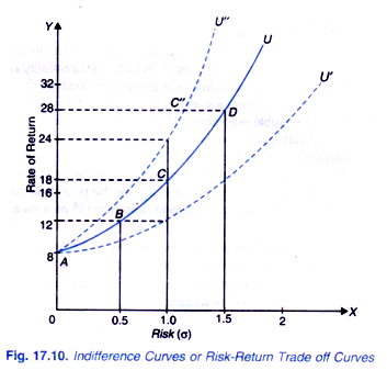
The concept of indifference curve or risk-return trade-off function can be better explained with Fig. 17.10 where on the X- axis, we measure risk in terms of standard deviation (σ) of probability distribution, and rate of return as per cent of investment is measured along the Y-axis.

An upward-sloping solid curve AU has been drawn from point A. Point A represents risk- free return of 8 per cent. This AU curve represents the risk-return trade off function of an individual or a firm and shows that 4 per cent extra return over and above risk-free return of 8 per cent is required to compensate him for the degree of risk given by σ = 0.5 (Note that 12 -8 = 4).

Here 8 per cent is a risk-free return as corresponding to it standard deviation (σ), which measures the level of risk, is zero. The difference between the required rate of return on a risky investment and the return on risk-free investment is called risk premium. Thus in the trade-off curve AU rate of return of 4 per cent is required on an investment with a risk of σ = 0.5.

Similarly, as will be seen from AU trade off curve in Figure 17.10 that to compensate the individual for undertaking an investment with a risk of σ = 1.0, return of 18 per cent is required (that is, risk premium on this investment is 10 per cent, 18 – 8 = 10). 28 per cent rate of return is required or expected on risky investment with σ = 1.5.

For a more risk-averse individual the higher rate of return is required for a risky investment with a given standard deviation. Therefore, for a more risk-averse manager risk-return trade­off curve will be steeper than AU curve. Thus, with a more risk-averse individual, a steeper indifference curve or risk-return trade-off curve AU” (dotted) has been drawn. With AU” risk- return trade off curve to compensate for risky investment with σ = 1.0, 24 per cent return is required, that is, his risk premium is 16 per cent as compared to 10 per cent of the previous individual.

Similarly, for a less risk-averse individual trade-off curve will be less steep such as AU (dotted). A individual with trade off curve AU’, to compensate him for risky investment with σ = 1.0, return of 12 per cent is required, (that is, 4 per cent risk premium is needed for a risk of σ = 1.0).

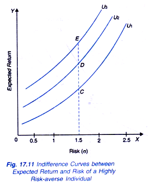
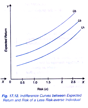
It is evident from above that different individuals will have different indifference curves between expected return and degree of risk depending upon their risk aversion. The individuals who are highly risk averse have more steeply indifference curves as shown in Fig. 17.11 and those who are less risk-averse they have flatter indifference curves as shown in Fig. 17.12.

 

It should be understood why we get higher indifference Curves such as U₂, U₃, of the individuals. When with a given degree of risk such as 1.5 σ in Fig. 17.11 expected return from investment increases the individuals shifts from a point C on indifference curve U₁ to point D on the higher indifference curve U₂. The similar reasoning holds good in case of individuals with flatter indifference curves. It needs to be re-emphasised that it is differences in attitudes towards risk of various individuals that make their indifference curves between risk and return of different slopes and concavity.

The Choice of an Investment Portfolio:

The individuals try to reduce risk by diversification. Towards that end the firms produce different types of products, that is, invest in different lines of business. Similarly, individuals investors choose a portfolio of assets to reduce overall risk of their investment.We have explained above how risk is measured by standard deviation and risk- return trade off curve is obtained. Now, the investors choose a risky portfolio of assets if it provides them adequate return.

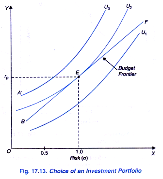
To explain the choice of an optimum portfolio we need another concept generally called a budget frontier. A budget frontier which represents the combinations of risk and return that are obtainable with the given available funds from mixed portfolios of two assets, say, shares of Reliance Industries and Tata Steel.

Suppose the expected returns from these assets are 20 per cent and 10 per cent respectively. If a portion W_i of the given available funds are invested in Reliance Industries and the remaining funds W_t are invested in Tata Steel, the expected return of the portfolio of these two assets is given by

r_p =W_ir_i+ W_t.rt …(1)

Where r_p = expected return of the portfolio of two assets.

r_i = the expected return of investment in Reliance Industries

r_t = the expected return from Tata Steel.

W_i = the proportion of the given funds invested in Reliance Industries

W_i = the remaining portion of the given funds invested in Tata Steel.

Note that W_i + W_t = 1 and different portfolios or combinations of two assets will involve different degrees of risk (a) and also yield different returns. Note that rate of return from a portfolio is the weightage average of the returns from the two assets as given by equation (1).

It is worth noting that any linear weighted combinations of returns from two assets with the given returns, r_i and r_t shows the rate of return from a portfolio of these two assets. We draw in Figure 17.13 such a budget frontier BF which shows the combinations or portfolios of two assets which are obtainable with the given funds.

It will be seen from Figure 17.13 that budget frontier BF is tangent to the trade-off function curve U₂ at point E which represents the optimum portfolio of two assets which yield return of r_p and involve a risk (σ) of 1.0. The combination of two assets represented by E is an optimally diversified portfolio containing a mix of the two assets.

If the rate of return on shares of Reliance Industries is 20 per cent and return on Tata Steel shares is 10 per cent. Suppose in the optimum portfolio, the individual spends 40 per cent of its investible funds on shares of Reliance Industries and the remaining 60 per cent on shares of Tata Steel, the rate of return on the portfolio can be calculated as follows

r_p = W_r r_i + W_tr_t

= 0.40 X 20 + 0.60 X 10

= 8 + 6 = 14

Thus rate of return of the portfolio of the two assets is 14 per cent.