In this essay we will discuss about monopoly market. After reading this essay you will learn about: 1. Meaning of Monopoly 2. Sources and Types of Monopoly 3. Monopoly Price Determination 4. Degree of Monopoly Power – Its Measure 5. Meaning of Monopoly Price Discrimination 6. Types of Price Discrimination 7. Conditions for Price Discrimination 8. Benefits of Price Discrimination and Other Details.
Contents:
- Essay on the Meaning of Monopoly
- Essay on the Sources and Types of Monopoly
- Essay on Monopoly Price Determination
- Essay on the Degree of Monopoly Power – Its Measure
- Essay on the Meaning of Monopoly Price Discrimination
- Essay on the Types of Price Discrimination
- Essay on the Conditions for Price Discrimination
- Essay on the Benefits of Price Discrimination
- Essay on the Harms of Price Discrimination
- Essay on Control and Regulation of Monopoly
Essay # 1. Meaning of Monopoly:
Monopoly is a market situation in which there is only one seller of a product with barriers to entry of others. The product has no close substitutes. In the words of Salvatore, “Monopoly is the form of market organisation in which there is a single fir m selling a commodity for which there are no close substitutes.”
The cross elasticity of demand with every other product is very low. This means that no other firms produce a similar product. Thus, the monopoly firm is itself an industry and the monopolist faces the industry demand curve. The demand curve for his product is, therefore, relatively stable and slopes downward to the right, given the tastes and incomes of his customers.
ADVERTISEMENTS:
It means that more of the product can be sold at a lower price than at a higher price. He is a price-maker who can set the price to his maximum advantage. However, it does not mean that he can set both price and output. He can do either of the two things. His price is determined by his demand curve, once he selects his output level.
Or, once he sets the price for his product, his output is determined by what consumers will take at that price. In any situation, the ultimate aim of the monopolist is to have maximum profits.
Essay # 2. Sources and Types of Monopoly:
Monopoly may arise from a number of sources and is of various types:
First, grant of a patent right to a firm by the government to make, use or sell its own invention.
ADVERTISEMENTS:
Second, control of a strategic raw material for an exclusive production process.
Third, a natural monopoly enjoyed by a firm when it supplies the entire market at a lower unit cost due to increasing economies of scale, just as in the supply of electricity, gas, etc.
Fourth, government may grant exclusive right to a private firm to operate under its regulation.
Such privately owned and government regulated monopolies are mostly in public utilities and are called legal monopolies such as in transport, communications, etc.
ADVERTISEMENTS:
Fifth, there may be government owned and regulated monopolies such as postal services, water and sewer systems of municipal corporations, etc.
Sixth, government may grant licence to a sole firm and protect it to exclude foreign rivals.
Seventh, the sole manufacturer of a product may adopt a limit pricing policy in order to prevent the entry of new firms.
Essay # 3. Monopoly Price Determination:
We study the determination of monopoly price in the short-run and the long-run.
It’s Assumptions:
The analysis of the determination of the price, output and profits under monopoly is based on the following assumptions:
(1) There is one seller or producer of a homogeneous product.
(2) There are no close substitutes for the product.
(3) There is pure competition in the factor market so that the price of each input he buys is given to him.
ADVERTISEMENTS:
(4) The monopolist is a rational being who aims at maximum profit with the minimum of costs.
(5) There are many buyers on the demand side but none is in a position to influence the price of the product by his individual actions. Thus the price of the product is given for the consumer.
(6) The monopolist does not charge discriminating price. He treats all consumers alike and charges a uniform price for his product.
(7) The monopoly price is uncontrolled. There are no restrictions on the power of the monopolist.
ADVERTISEMENTS:
(8) There is no threat of entry of other firms.
Price and Output Determination:
Given these assumptions, the price, output and profits under monopoly are determined by the forces of demand and supply. The monopolist has complete control over the supply of the product. He is also a price- maker who can set the price to his maximum advantage. But he cannot fix the price and output simultaneously.
Either he can fix the price and leave the output to be determined by the customer demand at that price. Or, he can fix the output to be produced and leave the price to be determined by the consumer demand for his product. Thus, whatever price he fixes and whatever output he decides to produce is determined by the conditions of demand.
ADVERTISEMENTS:
The demand curve faced by a monopolist is definite and is downward sloping to the right. It is his average revenue curve (AR). Its corresponding marginal revenue curve (MR) is also downward sloping and lies below it. But the manner and extent to which the monopolist will be able to influence price or output will depend upon the elasticity of demand for his product.
If the demand for his product is highly elastic, he can sell more by a small reduction in price. If, on the other hand, the demand is less elastic, the tendency will be to raise the price and profit more by selling less.
Given the demand for his product, the monopolist can select the most profitable output against this demand. His cost of production may be rising, falling or constant. Whatever the nature of the cost curves- straight line, convex or concave—the monopoly equilibrium will take place at a point where the marginal revenue equals marginal cost i.e. ƏR /ƏQ = ƏC /ƏQ.
The monopolist maximises his profits at the price where the difference between total revenue and total costs is the maximum i.e. Max π = TR-TC.
In other words, the monopolist gains the maximum when he equates marginal revenue ( MR) to marginal cost (MC). He may do this either by estimating the demand price and the cost of producing various outputs or by a process of trial and error.
Geometrically speaking, the point of monopoly equilibrium is one where the MC curve cuts the MR curve from below or from the left, and a perpendicular from it to the AR curve determines price.
ADVERTISEMENTS:
It implies that
Price > MC = MR. In fact, monopoly price = MC –E/E-1.
AR (Price) = MR MC –E/E-1 and MC = MR
Monopoly Price = MC E/E-1
Thus monopoly price is a function of the MC and the elasticity of demand. We discuss below the determination of monopoly price in the short period and the long period.
(A) Short-Run Monopoly Equilibrium:
ADVERTISEMENTS:
In the short-run, the monopoly firm attains equilibrium when its profits are maximised or losses are minimised. Like the competitive equilibrium, this analysis can also he discussed in terms of the total revenue-total cost approach and the marginal revenue-cost approach.
Total Revenue-Cost Approach:
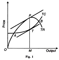
In Figure 1. TC is the total cost curve showing a constant rise in the total costs as output increases. TR is the total revenue curve which goes on rising to begin with, then flattens and later on slopes downward, showing fall in total receipts after a given point.
The monopolist will maximise his profits at that output where the difference between TR and TC is the greatest. This will be the level at which the slopes of TR and TC curves equal. Accordingly, P is the equilibrium point as determined by the tangents at points P and T on the TR and TC curves respectively.
A and В are the break-even points where TR = TC. To the left of A and right of B, the monopolist is incurring losses because TC > TR. Thus his maximum profits will be PT and he will sell OM output at MP Price.
ADVERTISEMENTS:
Marginal Revenue-Marginal Cost Approach:
In the short-run, the monopolist can change the price as well as the quantity of the product. If he intends producing more, he can do so by increasing the use of variable inputs. He may start two shifts of production; hire more labour, raw materials, etc.
But he cannot change his fixed plant and equipment. On the other hand, if he wants to restrict his output, he may dispense with certain workers, work for less hours and use less of the variable factors.
In any case, his price cannot be below the average variable costs. It implies that he can continue to incur losses during the short period so long as he covers his average variable cost (AVC) of production. Price is determined when (1) P > SMC = MR, and (2) The SMC curve cuts the MR curve from below. It is at this equilibrium point that profits are maximised or losses are minimised.
Super-normal Profits:
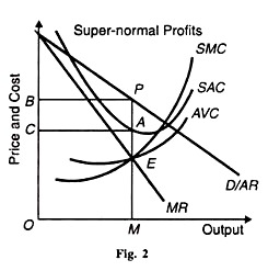
In Figure 2, SAC and SMC are the short-run average and marginal revenue curves respectively. AVC is the average variable cost curve. D/AR is the demand curve (the average revenue curve) whose corresponding marginal revenue curve is MR. The short-run monopoly equilibrium is at point E where the SMC curve cuts the MR curve from below.
The monopolist sells OM output at MP (=OB) price. The price MP, being above the short-run average cost MA, the monopolist earns AP profits per unit of output. Thus total monopoly profits are AP × CA= CAPB.
Normal Profits:
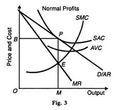
In Figure 3, the short-run equilibrium of the monopolist is shown when he earns only normal profits. The equality of SMC curve and MR curve at point E determines OM output which is sold at MP Price. Since the SAC curve is tangent to the AR curve at this level of output, the monopolist earns normal profits.
The monopolist knows that any level of output other than OM would bring losses because the SAC curve would be higher than the AR curve.
Minimum Losses:
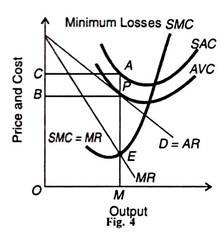
Figure 4 shows a short-run situation in which the monopolist incurs losses. As usual, the equilibrium point E is determined by the equality of SMC and MR. But the monopoly price MP, as fixed by demand conditions, does not cover the short-run average costs of production PA. It just covers the average variable costs MP, represented by the tangency of the demand curve D and the AVC curve at point P.
PA is thus per unit loss which the monopolist incurs. Total losses are equal to BP x PA = BPAC. In this figure, P is the shutdown point for this firm. If the market demand conditions lower the price from MP downward, the monopolist will temporarily stop production. His firm will close down.
(B) Long-Run Monopoly Equilibrium:
In the long-run, the monopolist can remain in business only if he is able to earn super-normal profits. If he was incurring losses in the short-run, he has enough time to make changes in his existing plant in the long- run so as to maximise his profits. With entry of new firms ruled out, he can install a plant which gives him maximum profits.
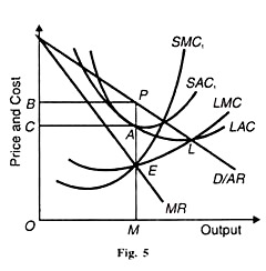
The scale of his plant depends upon the position of the demand (AR) curve and its corresponding MR curve. The most profitable level of output is at the point where the LMC curve intersects the MR curve from below and the SMC curve passes through this point. Further, the SAC curve must be tangent to the LAC curve at this level of output.
Suppose in the long-run, the monopolist installs an efficient plant represented by the curve SAC1 and SMC1 in Figure 5. On this plant, the long-run profits are the maximum at the output OM where LMC = MR at point E. Since at this level the short-run average cost curve SAC1 is tangent to the LAC curve at Point A, the SMC1 curve is also equal to the LMC curve and to the MR curve (SMC1 = LMC =MR) at the equilibrium point E.
Thus when the monopoly firm is in long-run equilibrium, it is also in short- run equilibrium. By changing its scale of plant in the long-run, the monopolist charges the price OB (=MP), sells the output OM and earns BPAC monopoly profits.
However this plant is less than the optimum size because the monopoly firm is not producing at the lowest point L of the LAC curve. It has some excess capacity. It is not in a position to take full advantage of the economies of scale due to the small size of the market for his product.
Essay # 4. Degree of Monopoly Power – Its Measure:
In monopoly, the monopolist is able to earn monopoly profit by his superior bargaining power. He is in a better position to exploit the market to his advantage. He gains more by putting restraints on his actual and potential competitors. Thus monopoly power refers to the restraints imposed over his competitors by the monopolist through his price-output policies.
Measurement of Monopoly Power:
There are two important methods of monopoly power:
First, the difference between marginal cost and price. Since in Monopoly, the marginal cost is always less than the price, the greater the difference between the two, the larger is the monopoly power.
Second, the difference between monopoly super-normal profits and competitive super-normal profits is also considered as the measure of monopoly power. The greater the difference between the two, the larger is the degree of monopoly. However, economists have given other measures of monopoly power. We discuss a few. But no method is regarded as perfect.
1. Lerner’s Measure:
One of the earliest methods to measure monopoly power is expressed by Prof. Abba P. Lerner in terms of the bargaining strength. The difference between price and marginal cost is the measure of the degree of monopoly power.
If P is price and MC the marginal cost, the formula for measuring the degree of monopoly power is P-MC/P. A seller’s monopoly power depends upon his ability to sell his product at a price much above his marginal cost.
The larger the gap between price and marginal cost, the greater is the monopoly power. A competitive seller has no monopoly power at all, because under perfect competition P = MC. In all cases, the above formula will give zero. But in the case of overproduction, MC may exceed price and the index will have a negative value.
Moreover, if the seller is a monopolist, the difference between price and marginal cost is always there. The index of monopoly power will, therefore, vary between zero and unity. For instance, if P is Rs.4 and MC Rs.2 the index of monopoly power will be 1/2 i.e. (4-2)/4.
It is, however, not easy for a seller to raise the price of his product in order to increase his bargaining price. The attempt to raise profits by a price rise may be neutralized by the reduction in his sales resulting from raising the price. Therefore, the degree of monopoly power is measured in terms of the elasticity of demand and the formula is:
Degree of monopoly power (DMP) = (P – MC)/ P
For profit maximisation, MC = MR, and the formula becomes
DMP= or the inverse of the elasticity of demand,
P- MR= (P – MR)/ P
By substituting MR = P E-1/E in the above equation,
DMP= (P-P E-1/E)/P = P- PE +P/E/P = PE- PE+P/EP = 1/E
Or the inverse of the elasticity of demand, P/P-MR
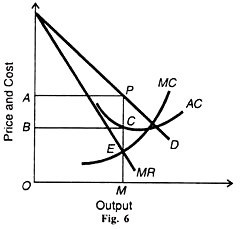
Lerner’s measure is illustrated in Figure 6 where AC and MC curves are the firm’s average and marginal cost curves, while D and MR are its demand and marginal revenue curves. The monopolist firm maximizes its profit at point E where MC = MR.
It produces OM output and sells it at MP Price. The ratio PEIPM is termed as the degree of monopoly power. The degree of monopoly power is the reciprocal of the P-MR elasticity of demand i.e., P-MR/P
In Figure 6, P is equal to PM while MR is equal to EM.
Rewrite the formula,
DMP = P-MR/P
= PM-EM/PM
DMP = PE/PM
The formula indicates that the degree of monopoly power is the reciprocal of the price elasticity of demand E. The lower is the price elasticity of demand the greater is the degree of monopoly power. The higher the elasticity, lower the monopoly power.
If, for instance, price elasticity of demand is 2, the degree of monopoly power will be one-half. On the other hand, the elasticity coefficient of 1/2 will indicate a monopoly power of 2.
Its Limitations:
Though interesting, this measure of monopoly power has many limitations. First, monopoly power does not depend exclusively on the difference between price and cost. It also depends on the restriction of output by the monopolist seller.
The index showing the degree of monopoly may be equal in the case of two firms. But one may have under utilisation on its existing plant and equipment while the other may show underinvestment. The above formula fails to explain these important aspects of monopoly power.
Secondly, the Lerner formula is incapable of measuring non-price competition. Again the index of monopoly power may be the same in case of two firms. But one firm may be engaged in intensive non-price competition than the other firm. It may thus be selling a large quantity of its product. Lerner’s formula does not throw any light on this aspect of the problem.
Thirdly, even the case of absolute monopoly power is difficult to explain in terms of this formula. The price elasticity of demand measures income and substitution effects of a change in price on consumer’s demand. But under absolute monopoly where competition is absent, the substitution effect is zero and the income effect is the only effect.
Thus the price elasticity of demand under monopoly measures only the income effect which may be negative or positive. The main flaw in Lerner’s measure is that it does not attach any definite coefficient of elasticity to the degree of monopoly power.
Fourthly, Lerner’s measure is essentially static. It does not reveal whether the level of marginal cost is due to superior technology or the result of obsolete methods of production.
Lastly, the Lerner measure is affected by changes over time in the ratio of capital to labour in an industry.
Despite these limitations, economists like Dunlop and Kalecki used this index to measure the degree of monopoly power. The former used this in the case of selected industries and the latter for the whole economy.
2. Triffin’s Measure:
Prof. Robert Triffin has improved upon Lerner’s measure by suggesting price cross-elasticity instead of price elasticity of demand. Price cross-elasticity of demand measures the degree of substitution between the products of two firms when a change in the price of one firm’s product affects the demand for the other’s product.
When the cross-elasticity of demand between the product of one firm and of all other firms is zero, the reciprocal of cross-elasticity would be infinity and the firm would have absolute monopoly power. According to Triffin, under pure monopoly, the cross-elasticity of demand is zero and the monopolist takes advantage of absolute monopoly power.
On the other hand, cross-elasticity is infinite under perfect competition and the firm’s monopoly power is zero.
Its Criticisms:
First, like Lerner’s measure, the Triffin measure is unsuitable for practical purposes. Pure monopoly like pure competition is unreal. Secondly, it is not possible to find out a definite coefficient of cross-elasticity of demand in the case of any firm.
Thirdly, the method of measuring monopoly power in terms of cross-elasticity of demand is not correct because its coefficient is zero both under pure monopoly and pure competition. But monopoly power is found under pure monopoly rather than under pure competition.
3. Bain’s Measure:
Prof. J.S. Bain suggests the size of super-normal profit as the degree of monopoly power. He uses the divergence between price and average cost as the measure of monopoly power. Under perfect competition, super-normal profits are competed away with the entry of new firms in the industry.
So the degree of monopoly power is zero when competition is pure. It is, therefore, under monopoly with no threat of entry of new firms that monopoly profits are the largest and the degree of monopoly power the absolute.
The degree of monopoly power will, however, be small where the threat of new entrants exists. Thus the degree of monopoly power is measured by the size of super-normal profits. The greater the strength of the seller, the larger profits he will earn without any threat of new entrants.
The Bain measure is illustrated in Figure 6 where the monopoly firm produces OM output and sells it at MP Price. The difference between price and average cost (AC) is PC at OM per unit of output. Thus A PC В are the super-normal profits which measure monopoly power.
It’s Shortcomings:
But this measure is also not free from shortcomings.
First, it is difficult to estimate the net income accruing to a firm. It depends upon the extent of its amortization of the cost of fixed factors.
Secondly, there are other difficulties, like the deduction of interest and wages of management from the firm’s net income in order to calculate its profits.
Thirdly, all profits accruing to a firm are not monopoly profits. Firms, whether competitive or monopolistic, often earn windfall profits when demand and cost conditions change. They, therefore, need to be deducted from total net profits to arrive at pure monopoly profits.
Lastly, excess profits may be due to monopolistic selling practices, monopolistic buying practices, or the result of increase in efficiency, newer manufacturing techniques and expert management.
4. Rothschild’s Measure:
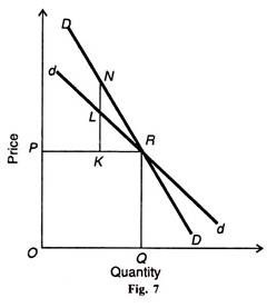
Prof. Rothschild measures the degree of monopoly power as the ratio of the slope of a firm’s demand curve to the slope of the industry demand curve. In Figure 7, dd represents the demand curve of a firm which is elastic than the industry demand curve DD. Thus
DMP=Slope of dd/Slope of DD= (KL/KR)/(KN/KR) = KL/KN
Since under pure competition the demand curve of a firm is horizontal, the Rothschild index equals zero. Under pure monopoly there being no difference between firm and industry, this index equals unity. Therefore, the degree of monopoly power exists between zero and unity.
It’s Weaknesses:
The Rothschild measure of the degree of monopoly power is vaguer than the other measures.
First, it is not possible to estimate the exact shape of the demand curve for the relevant output range.
Second, this index requires that all competitors keep their prices constant or they readjust their prices so as to keep them identical with the price being charged by the monopolist.
Lastly, this measure is based exclusively on demand factors and neglects supply and cost conditions.
Essay # 5. Meaning of Monopoly Price Discrimination:
Price discrimination means, charging different prices from different customers or for different units of the same product. In the words of Joan Robinson: “The act of selling the same article, produced under single control at different prices to different buyers is known as price discrimination.”
Price discrimination is possible when the monopolist sells in different markets in such a way that it is not possible to transfer any unit of the commodity from the cheap market to the dearer market.
Price discrimination is, however, not possible under perfect competition, even if the two markets could be kept separate. Since the market demand in each market is perfectly elastic, every seller would try to sell in that market in which he could get the highest price. Competition would make the price equal in both the markets. Thus price discrimination is possible only when markets are imperfect.
Essay # 6. Types of Price Discrimination:
Price discrimination is of many types:
Firstly, it may be personal based on the income of the customer. For example, doctors and lawyers charge different fees from different customers on the basis of their incomes. Higher fees are charged to rich persons and lower to the poor.
Secondly, price discrimination may be based on the nature of the product. Paperback is cheaper than the deluxe edition of the same book, for the former is bought by the majority of readers, and the latter by libraries. Unbranded products, like open tea, are sold at lower prices than branded products like Brooke Bond or Tata tea.
Economy size tooth pastes are relatively cheaper than ordinary-sized tooth pastes. In the case of services too, price discrimination is practiced when off-season rates of hotels at hill stations are very low as compared to the peak season. Dry-cleaning firms charge for two while they clean three clothes during off-season; whereas they charge more for quick service in peak season.
Thirdly, price discrimination is also related to the age, sex and status of the customers. Barbers charge less for children’s haircuts.
Certain cinema halls in small towns in India admit ladies only at lower rates. Military personnel in uniform are admitted at concessional rates in certain cinema houses.
Fourthly, discrimination is also based on the time of service. Cinema houses at certain places, like New Delhi, charge half the rates in the morning show than in the afternoon shows.
Fifthly, there is geographical or local discrimination when a monopolist sells in one market at a higher price than in the other market.
Lastly, discrimination may he based on the use of the product. Railways charge different rates for different compartments or for different services. Less is charged for the transportation of coal than for bales of cloth on the same route. State power boards charge low rates for industrial use than for domestic consumption of electricity.
Essay # 7. Conditions for Price Discrimination:
For price discrimination to exist the following conditions must be satisfied:
(1) Market Imperfections:
Price discrimination is possible when there is some degree of market imperfection. The individual seller is able to divide and keep his market into separate parts only if it is imperfect. Customers do not move readily from one market to the other because of ignorance or inertia.
(2) Agreement between Rival Sellers:
Price discrimination also takes place when the seller of a commodity is a monopolist or when rivals enter into an agreement for the sale of the product at different prices to different customers. This is usually possible in the sale of direct services.
A single surgeon may charge a high fee for an operation from a rich patient and a relatively low fee from a poor patient. Lawyers charge from their clients in proportion to the degree of risk or amount of money involved in a law suit. Price discrimination is possible in the case of services because there is no possibility of resale.
(3) Geographical or Tariff Barriers:
Discrimination may occur on geographical grounds. The monopolist may discriminate between home and foreign buyers by selling at a lower price in the foreign market than in the domestic market. This type of discrimination is known as “dumping”.
It can only be successful if the commodities sold abroad can be prevented from being returned to the home country by tariff restrictions. Sometimes transport costs are so high that they act as a safeguard against the return of dumped goods.
(4) Differentiated Products:
Discrimination is possible when buyers need the same service in connection with differentiated products. Railways charge different rates for the transport of coal and copper. For they know that it is physically impossible for a copper merchant to convert copper into coal for the purpose of transporting it cheaper.
It also applies to discrimination based on age, sex, status and income of buyers of services. For instance, a rich man cannot become poor for the sake of getting cheap medical facilities.
(5) Ignorance of Buyers:
Discrimination also occurs when small manufacturers sell goods made to order. They charge different rates to different buyers depending upon the intensity of their demand for the product. Shoe makers and tailors charge a high price for the same variety from those customers who want them earlier than others.
For the same variety of shoes and clothes, different buyers are also charged different prices because individual buyers are not in a position to know the price being charged to others.
(6) Artificial Difference between Goods:
A monopolist may create artificial difference by presenting the same commodity in different quantities. He may present it under different names and labels, one for the rich and snobbish buyers and the other for the ordinary.
Thus he may charge different prices for substantially the same product. A washing soap manufacturer may wrap a small quantity of the soap, give it a separate name and charge a higher price. He may sell it at Rs.20 per kg. as against Rs.18 for the unwrapped soap.
(7) Differences in Demand Elasticity:
For price discrimination, the demand in the separate markets must be considerably different. Different prices can be charged in separate markets based on differences of elasticity of demand. Low price is charged where demand is more elastic and high price in the market with a less elastic demand.
(4) Price Determination under Monopoly Discrimination:
Price discrimination occurs when the monopolist divides the buyers of his commodity or service into two or more groups and charges a different price to each group. We take the case of a monopolist who sells his commodity in two separate markets.
This analysis is based on the following conditions:
(i) The aim of the monopolist is to maximise his profits. He, therefore, produces that output at which his marginal revenue equals marginal cost. Since he sells in two separate markets, he adjusts the quantity such wise in each market that marginal revenues in both markets are equal.
Given the marginal cost of producing the commodity, the most profitable monopoly output will be determined at a point where the combined marginal revenue of both the markets equals the marginal cost.
Or, monopoly profit = MR1 = MR2 = MC. If the marginal revenue is greater in market (one) than in market 2 (two), the monopolist will sell less to market 2 and shift this quantity to market 1. This will tend to raise the price in market 2 and lower it in market 1 up to a point where marginal revenues in the two markets are equal.
(ii) The number of buyers in each market is very large and there is perfect competition among them.
(iii) There is no possibility of resale from one market to the other.
(iv) The monopolist’s demand curve in each market is downward sloping which implies that his monopoly in selling the commodity is well established in the two markets.
(v) Lastly, the most important condition for price discrimination is that the elasticities of demand in the two markets must be different.
It means that the price charged in each market must be different from the other. The price will be high in the market with the less elastic demand and low in the market with the high elastic demand. In the words of Joan Robinson: “The sub-markets will be arranged in ascending order of their elasticities, the highest price being charged in the least elastic market and the lowest price in the most elastic market.”
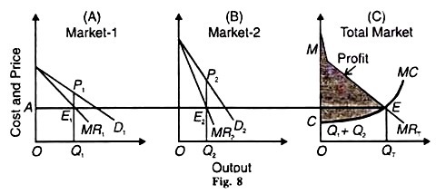
Figure 8 illustrates price and output determination under price discrimination. The monopolist sells his product in two markets, 1 and 2. Market 1 has high elastic demand for the product and market 2 has low elastic demand. Accordingly, the demand curve in market 1 is D1 and its corresponding marginal revenue curve is MR1 and in market 2 the corresponding curves are D2 and MR2.
Panel С of the figure shows MRT, the total marginal revenue curve, drawn by the lateral summation of MR1, and MR2, curves, and MC is the marginal cost curve. The point of intersection between the MRT and MC curves at E determines the equilibrium level of output OQT.
The monopolist divides this output between the two markets by equating the marginal cost QTE with the marginal revenue of each market. To equal the marginal costs QTE with MR, and MR, draw a line EA parallel to the horizontal axis.
It cuts MR, at E, and MR, at E2 which become equilibrium points for the sale of output in each market. Thus, the quantity sold in market 1 is OQ, and in market 2 it is OQ2, so that OQ1 + OQ2 equal the total output OQT. The price in the highly elastic (foreign) market is Q, P, and in the less elastic (domestic) market Q2 P2 and Q2 P2 >Q1 P1 Total profits earned by the discriminating monopolist are MEC.
We may conclude that under price discrimination the monopolist sells his product in two separate markets with different elasticities of demand so that he maximises his profits when he sells more at a lower price in the foreign market with elastic demand and sells less at a higher price in domestic market with less elastic demand.
It follows that when marginal revenues equal and prices differ in the two markets, price discrimination is possible and profitable.
(5) Dumping: International Price Discrimination:
Dumping is international price discrimination in which an exporter firm sells a portion of its output in a foreign market at a very low price and the remaining output at a high price in the home market. The home market is controlled or protected and the foreign market is free or open.
Heberler defines dumping as:
“The sale of goods abroad at a price which is lower than the selling price of the same goods at the same time and in the same circumstances at home, taming account of differences in transport costs.”
Its Assumptions:
The analysis of price-output determination under dumping assumes that:
(a) Total output is not fixed, it can be varied;
(b) Marginal revenues must be equal in the two markets, and
(c) The foreign market is perfectly competitive and the home market is monopolistic, so that the demand curve facing the monopolistic in the foreign market is perfectly elastic and in the home market less elastic.
Explanation:
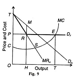
Given, the above assumptions, price, output will be determined by the equality of the total marginal revenue curve and the marginal cost curve of producing the commodity. Figure 9 illustrates price-output determination under dumping. The foreign market demand curve faced by the monopolist is the horizontal line PDF which is also the MR curve because the foreign market is assumed to be perfectly elastic.
The demand curve in the home market with a less elastic demand for the product is the downward sloping curve DH and its corresponding marginal revenue curve is MR^ The lateral summation of the MRH and PD curves leads to the formation of TREDF as the combined marginal revenue curve.
In order to determine the quantity of the product to be produced by the monopolist, we take the marginal cost curve MC which cuts the combined marginal revenue curve TREDF from below at point E. Thus OF output will be produced for sale in the two markets.
Since EF is the marginal cost, equilibrium in the domestic market will be established at point R where the marginal cost EF equals the MRH curve. Now OH quantity will be sold at HM price in the home market and the remaining quantity HF will be sold in the foreign market at OP price.
Thus the monopolist sells more in the foreign market with the more elastic demand at a low price and less in the home market with the less elastic demand at a high price. His total profits are TREC.
Essay # 8. Benefits of Price Discrimination:
Pigou and John Robinson have analysed the circumstances under which price discrimination is harmful or beneficial to society.
a. Benefits to Society:
In many cases where there is perfect competition or simple monopoly, production of a certain commodity is not possible because its average cost curve lies above its demand (AR) curve. But under price discrimination the average cost curve is likely to be below the average revenue curve at some point. Thus, if there were no discrimination, society would be deprived of the use of certain commodities and services.
As emphasised by Mrs. Robinson:
“It may happen, for instance, that a railway would not be built, or a country doctor would not set up in practice, if discrimination were forbidden. From the point of view of society, it is only necessary that the concern should make sufficient profits to maintain the efficiency of the plant, and not a profit which would have been sufficient to justify the original investment.”
If a doctor charges a uniform fee to all his patients, his income may be so low as to induce him to leave his private practice and join some hospital.
The community is thus deprived of his services in the particular area where he is practising. If, however, he charges more fee to his rich patients than to the ordinarily, his income is likely to be so high as to induce him to stay in that area. Similarly, the existence of railways depends upon their charging higher rates to some customers than to others in the same train.
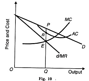
If discrimination occurs under conditions of falling average costs, it is actually beneficial to consumers because it results in larger output for the market. This is illustrated in Figure 10 where D is the average revenue curve of the discriminating monopolist and d/MR is the ordinary demand curve which becomes the MR curve to the discriminator.
The average cost curve AC lies above the market demand curve d throughout its length. So no production is possible at any price on the ordinary d curve. But production is possible under price discrimination because the demand curve D of the discriminating о monopolist lies above the downward sloping portion of the AC curve. Equilibrium is established at E where MC = MR and the output OQ is produced and sold at QP price and the discriminator g earns RP profits per unit of output.
b. Economic Welfare:
Price discrimination is justified if it helps in promoting economic welfare. Governments usually permit or even encourage price discrimination if it leads to the production of some public utility service, such as telephone, telegraph, or rail о transportation. In public utility services, the higher income groups are charged higher prices and the funds so collected may be used to subsidies the goods meant for the poor.
c. Reducing Inequalities:
Price discrimination is also beneficial to society for it helps in reducing inequalities of personal incomes when higher prices or fees are charged to the rich than to the poor. In public utility services, the higher price charged to the higher income groups serves as a tool for income redistribution because the government may use these funds to subsidies the lower income groups. Thus price discrimination helps in promoting social warfare.
d. Through Dumping:
Price discrimination is not only beneficial but is also justified when a country sells a commodity cheaper abroad than at home. If a foreign market is elastic, more will be sold at a lower price. It means expansion in output, the use of larger resources of the economy, more employment and income to the community.
Price discrimination of this type proves particularly useful if the industry obeys the law of decreasing costs. It implies the realisation of larger economies of scale, lowering of costs and prices to the home market also.
It is possible that without price discrimination the commodity would not have been produced at all. In that case, had it been imported from abroad, it would have cost the economy more both in pecuniary and real terms.
Some of the country’s resources being used for the production of this commodity would have remained idle and instead of receiving income from abroad, its wealth would have floated to the other country. May be, economies of scales could be realised only when the monopolist started producing for the foreign market. Hence price discrimination is justified.
Essay # 9. Harms of Price Discrimination:
a. Mal-Allocation of Resources:
Price discrimination is, however, harmful to society when it leads to mal-distribution of resources as between different uses with the result that output, employment and income are not maximised.
b. Diversion of Resources:
It may lead to the diversion of resources from their socially optimal uses.
c. Exploitation of People:
It leads to exploitation when people are made to pay higher prices for smaller quantities.
d. Harms of Dumping:
Even on international plane when price discrimination takes to form of dumping, it. Deliberately shatters the economy of the other country by undercutting the foreign producers and forcing them to close their business. Such discrimination is highly undesirable.
Essay # 10. Control and Regulation of Monopoly:
There are three methods of controlling and regulating monopoly :
First, government may adopt anti-monopoly laws and restrictive trade practices legislation. Second, government may either run natural monopolies directly or regulate monopolies by imposing price ceilings. Third, government may regulate monopolies through taxation.
Besides, there are certain fears that prevent the monopolist from charging a very high price in order to earn large super-normal profits. They are discussed as under.
(1) Fear of Potential Rivals. The fear of potential competitors may prevent a monopolist to charge a very high price to his customers. If he sets a vary high price, he will earn large super-normal profits. Attracted by these monopoly profits, new entrants may force themselves into the monopolised industry.
The monopolist, being averse to the entry of new firms, would prefer to charge a reasonable price and thus earn only a modest profit.
(2) Fear of Government Regulation. The same consideration applies to potential government regulation. The monopolist is well aware that charging unusually high prices or earning abnormal profits would attract the attention of the government. Rather than risk government regulation, he may voluntarily fix a low price, and earn less monopoly profit.
(3) Fear of Nationalisation. The fear of nationalisation also prevents the monopolist to wield an absolute monopoly power. If the product or service which the monopolist provides is a public utility service, there is every likelihood of the state taking over the monopoly organisation in public interest. This consideration may prevent the monopolist from charging too high a price.
(4) Fear of Public Reaction. The monopolist is also aware of public reaction if he charges a very high price and earns huge profits. Voices may be raised against the monopoly firm in parliament to press for anti- monopoly legislation.
(5) Fear of Boycott. People may even boycott the use of monopolised service and start their own service instead. For instance, if in a big city taxi operators combine to charge high rates, people may boycott taxi service and even start operating their own services by forming a cooperative society. Naturally, such a fear compels monopoly firms to charge reasonable prices and earn only nominal profits.
(6) Fear of Substitutes. Then there is the fear of substitutes. In fact, the fear of substitutes is the most potent factor which prevents monopoly firms from charging very high prices and thereby earn super-normal profits.
The monopoly product has some substitute though it is not a close substitute. Therefore, the fear of the emergence of very close substitutes is always uppermost in the mind of the monopolist which acts as a restraint on his absolute power.
(7) Differences in Elasticities of Demand. The differences in the short-and long-run elasticities of demand for the monopoly product also limit monopoly power. In the short-run, the monopolist can charge a very high price because customers take time to adjust their habits, tastes and incomes to some other substitutes.
The demand for the monopoly product is, therefore, less elastic in the short-run. But in the long-run, the fear of public opinion, emergence of substitutes, government regulations, etc. will force the monopolist to set a low price. He will view his demand curve as elastic, and sell more at a low price.”
(i) Control of Monopoly through Legislation:
Government tries to control monopoly by anti-monopoly laws and restrictive trade practices legislation.
These measures tend to:
(i) Remove restrictive trade practices and fixation of high prices;
(ii) Reduce the incidence of market-sharing agreements;
(Hi) Remove unfair competition;
(iv) Restrict the control of very large share of the market;
(v) Prevent unfair price discrimination;
(vi) Restrict mergers in order to avoid market domination; and
(vii) Prohibit exclusive agreements between the producer and retailer to the detriment of other traders.
(ii) Control of Monopoly through Price Regulation:
We now take the case where the government feels that monopoly price is very high and tries to bring it down by price regulation. To regulate monopoly, the government imposes price ceiling so that monopoly price should be near or equal to competitive price.
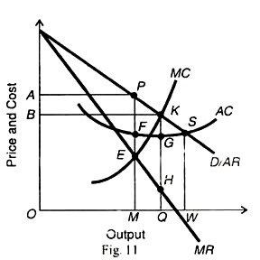
This is done when the government appoints a regulating authority or commission which fixes a price for the monopoly product below the monopoly price, thereby increasing output and lowering the price for the consumer. This is illustrated in Figure 11.
Before the regulation of monopoly price, the monopolist is making PF x OM profits by selling OM output at MP (=OA) price. Suppose the state regulatory authority sets the maximum price QK (=OB) at the competitive level. The new demand curve facing the monopolist becomes BKD. Its corresponding MR curve becomes BKHMR.
Now the monopolist behaves as a perfectly competitive producer. He produces and sells OQ output at point К where the MC curve cuts the BKHMR curve from below. As a result of price regulation, the monopolist increases his output to OQ from OM. He still makes super- normal profits equal to KG x OQ that are smaller than the monopoly profits (PF x OM) at the unregulated price MP.
If the price regulatory authority fixes the monopoly price WS equal to the average cost where the AC curve cuts the D/AR curve at point S, the monopolist would be able to place a greater quantity of output OW in the market.
At this level, the monopolist would earn only normal profits. In such a situation, the monopolist would continue to produce so long as he is getting a fair return on his capital investment. But the regulatory authority cannot force him to increase output beyond OW because the monopolist would not be operating at a loss.
(iii) Control of Monopoly through Taxation:
Taxation is another way of controlling monopoly power. The tax may be levied lump-sum without any regard to the output of the monopolist. Or, it may be proportional to the output, the amount of tax rising with the increase in output.
Lump-sum Tax:
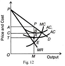
By levying a lump-sum tax, the government can reduce or even eliminate monopoly profits without affecting either the price or output of the product. A lump-sum tax imposed on the monopoly firm is shown in Figure 12 where AC and MC are the average cost and marginal cost curves before the tax is levied. The monopolist earns APRT super-normal profits by selling OM product at MP Price.
The imposition of the lump-sum tax is, in fact, a fixed cost to the monopoly firm because it is independent of output. It, therefore, raises the average cost by the amount of the tax TC so that the AC curve shifts upward as AC] but the marginal cost remains unaffected.
So the imposition of a lump-sum tax has the effect of reducing monopoly profit from APRT to APBC. The entire burden of the tax will be borne by the monopolist himself.
He cannot shift any part of it to his customers at any stage by raising the price and reducing output. Since the monopolist’s marginal cost curve and the marginal revenue curve remain unaffected by the tax imposition, any change in the existing price- output combination would only lead to losses.
Specific Tax:
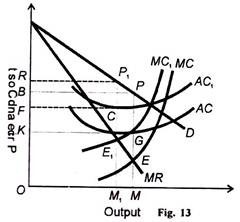
The government can also reduce monopoly profits by levying a specific or a per unit tax on the monopolist’s product. A per unit tax on monopoly output has the effect of shifting both the average and marginal cost curves upward by the amount of the tax.
Figure 13 illustrates this case. AC and MC are the monopoly firm’s average cost and marginal cost curves before the tax imposition. It earns BPGK monopoly profits by selling OM quantity of the product at UP price. Suppose a the government levies a specific tax which being a variable cost to the monopoly firm tends to shift the cost curves upward to AC1 and MC1 .
The monopolist’s new equilibrium point is E1 where the MC1 curve cuts the MR curve. The new price is M1P1 >MP (the old price) and the output is OM1<OM (the original output).
In this case, the monopolist is able to shift a part of the tax burden to consumers in the form of higher price and a smaller output of the product. Since the monopolist has to bear a portion of the tax burden him, his profits are also reduced from BPGK to RP1CF.
Such a tax does not help in regulating monopoly price and output. For the higher, the demand elasticity of tax, the higher the price for the product and the lower the output. The ultimate loss will be borne by the public rather than by the monopolist.
