Essay on Oligopoly: Top 8 Essays on Oligopoly | Markets | Microeconomics

Here is a compilation of essays on ‘Oligopoly’ for class 9, 10, 11 and 12. Find paragraphs, long and short essays on ‘Oligopoly’ especially written for school and college students.

Essay on Oligopoly

---

Essay Contents:

1. Essay on the Introduction to Oligopoly
2. Essay on the Characteristics of Oligopoly
3. Essay on the Scope of Study of Oligopoly
4. Essay on the Models of Oligopoly
5. Essay on the Sales (Revenue) Maximisation
6. Essay on the Constrained Revenue Maximisation
7. Essay on Game Theory
8. Essay on Payoff (Profit) Matrix

---

Essay # 1. Introduction to Oligopoly:

Two extreme market forms are monopoly (characterised by the existence of a single seller) and perfect competition (characterised by a large number of sellers). Competition is of two types- perfect competition and monopolistic competition. In perfect competition, all sellers sell ho­mogeneous products while in monopolistic competition they sell heterogeneous products. In monopoly there is no rival.

So the monopolist is not concerned with the effect of his actions on rivals. In both types of competition, the number of firms is so large that the actions of any one seller have little, if any, effect on its competitors. An industry with only a few sellers is known as an oligopoly, a firm in such an industry is known as an oligopolist.

Although car-wash is a million rupee business, it is not exactly a product familiar to most consumers. However, often many familiar goods and services are supplied only by a few com­peting sellers, which means the industries we are talking about are oligopolies. An oligopoly is not necessarily made up of large firms. When a village has only two medi­cine shops, service there is just as much an oligopoly as air shuttle service between Mumbai and Pune.

Essentially, oligopoly is the result of the same factors that sometimes produce monopoly, but in somewhat weaker form. Honestly, the most important source of oligopoly is the exist­ence of economies of scale, which give better producers a cost advantage over smaller ones. When these economies of scale are very strong, they lead to monopoly, but when they are not that strong they lead to competition among a small number of firms.

Since an oligopoly con­tains a small number of firms, any change in the firms’ price or output influences the sales and profits of competitors. Each firm must, therefore, recognise that changes in its own policies are likely to elicit changes in the policies of its competitors as well.

As a result of this interdependence, oligopolists face a situation in which the optimal deci­sion of one firm depends on what other firms decide to do. And so there is opportunity for both conflict and cooperation. Oligopoly refers to a market situation in which the number of sellers is few, but greater than one. A special case of oligopoly is monopoly in which there are only two sellers.

---

Essay # 2. Characteristics of Oligopoly:

The notable characteristics of oligopoly are:

1. Price-Searching Behaviour:

An oligopolist is neither a price-taker (like a competitor) nor a price-maker (like a monopolist). It is a price-searcher. An oligopolist is neither a big enough part of the market to be able to act as a monopolist, nor a small enough part of the market to be able to act as a competitor. But each firm is a dominant part of the market.

In such a situation, competition among buyers will force all the sellers to charge a uniform price for a product. But each firm is sufficiently so large a part of the market that its actions will have noticeable effects upon his rivals. This means that if a single firm changes its output, the prices charged by all the firms will be raised or lowered.

2. Product Characteristics:

In oligopoly, there may be product differentiation as in monopolistic competition (called differ­entiated oligopoly) or a homogeneous product may be traded by all the few dominant firms (as in pure oligopoly).

3. Interdependence and Uncertainty:

In oligopoly no firm can take decision on price independently. It is because the decision to fix a new price or change an existing price will create reactions among the rival firms. But rivals’ reactions cannot be predicted accurately. If a firm reduces its price its rivals may reduce their prices or they may not. So there is lack of symmetry in the behaviour of rival firms.

This type of reaction of rivals is not found in perfect competition or monopolistic competition where all firms change their price in the same direction and by the same magnitude in order to remain competitive and survive in the long run. So the outcome of a firm’s decision is uncertain.

For this reason it is difficult to predict the total demand for the product of an oligopolistic industry. It is still more difficult, and in some situations virtually impossible, to estimate the share of an individual firm in industry’s output.

It is true that the consequences of attempted price variations on the part of an individual seller are uncertain. His rivals may follow his change, or they may not, but they will, in all likelihood, notice it. The results of any action on the part of an oligopolist or even a duopolist depend upon the reactions of his rivals. In short, it is not possible to define general price- quantity relations for an individual firm, since reaction patterns of rivals are highly uncertain and almost completely unknown.

4. Different Reaction Patterns and Use of Models:

It is not true to say that, in oligopoly, profit is always maximised. It is because an oligopolist does not have control over all the variables which affect his profit. Moreover, a variety of possible reaction patterns is possible in this market—there is a conjectural variation in this market.

Just as firm A’s profit depends on the output of firm B also, firm B’s profit, in its turn, depends on firm A’s output. This is why various models are used to describe the diverse behaviour of oligopoly markets where a variety of outcomes is possible.

5. Non-Price Competition:

As in monopolistic competition there is not only price competition but non-price competition as well in oligopoly (and, to some extent, in duopoly). For example, advertising is often a life and death question in this type of market due to strategic behaviour of all firms. In most oligopoly situations we find intermediate outcomes. Economists are yet to emerge with a definite behaviour pattern in oligopoly.

---

Essay # 3. Scope of Study of Oligopoly:

Here we study a few of the many possible reaction patterns in duopoly and oligopoly situa­tions. The focus is on pure oligopoly. Here we assume that all firms produce a homogeneous product. We do not discuss the case of differentiated oligopoly and the issue of selling cost (advertising) separately. Of course, we discuss briefly Baumol’s sales maximisation hypoth­esis—without and with advertising.

The focus here is on the interdependence of the various sellers’ reactions, which is the essential distinguishing feature of oligopoly. If the influence of one seller’s quantity decision from the profit of another, δπ_i/δq_j, is negligible, the industry must be either perfectly competi­tive or monopolistically competitive. If δπ_i/δq_j, is perceptible, the industry is duopolistic or oligopolistic.

The optimum quantity and maximum profit of a duopolist or oligopolist depend upon the actions of the firms belonging to the industry. He can control only his own output level (or price, if his product is differentiated), but he has no direct control over other variables which are likely to (or do) affect his profits. In truth, the profit of each oligopolist is the result of the interaction of the decisions of all players in the market.

Since there are no generally accepted behavioural assumptions for oligopolists and duopolists as is found in other market forms, there are diverse patterns of behaviour and many different solutions for oligopolistic and duopolistic markets. Each solution is based on different types of models and each model is based on a different behavioural assumption or a set of assumptions.

Here we start with one or two simple duopoly models. The same analysis (solution) can be extended to cover any oligopolistic market. The earliest model of duopoly behaviour is the Cournot model, with which we may start our review of different oligopoly models. We end with the game theoretic treatment of oligopoly which shows decision-making under conflict.

---

Essay # 4. Models of Oligopoly:

1. The Cournot Model:

The Cournot model (presented in 1838) is based on the analysis of a market in which two firms produce a homogeneous product. Augustin Cournot (a French economist) noticed that only two firms were producing mineral water for sale. He argued that each firm would choose quan­tity that would maximise profit, taking the quantity marketed by its competitor as given.

Two main features of the model are:

(i) Each firm chooses a quantity of output instead of price; and

(ii) In choosing its output each firm takes its rival’s output as given.

In Cournot’s model, then, strategies are quantities of output. Here we assume that firms produce a homoge­neous good and know the market demand curve.

Each firm must decide how much to produce, and the two firms make their decisions at the same time. When taking its production decision, each duopolist takes into consideration its competitor. It knows that its competitor is also de­ciding how much to produce, and the market price will depend on the total output of both firms.

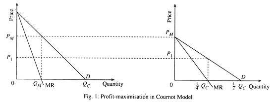
The essence of the Cournot model is that each firm treats the output level of its competitor as fixed and then decides how much to produce. Each Cournot’s duopolist believes that the other’s quantity will not change. In Fig. 1 when I produces Q_M, II maximises its profit by producing 1/4Q_C. In order to sell Q_M plus Q_c, the price must fall to P₁. Here Q_M is the mo­nopoly output which is half the competitive output Q_c.

The inverse demand function, stating price as a function of the aggregate quantity sold, is expressed as:

P =f (q₁) + q₂ … (1)

where q₁ and q₂ are the output levels of the duopolists. The total revenue of each duopolist depends upon his own output level as also as that of his rival:

R₁ = q₁f₁ (q₁ + q₂) = R₁ (q₁, q₂)

R₂ = q₂f₂ (q₁ + q₂) = R₂ (q₁, q₂) … (2)

The profit of each equals his total (sales) revenue, less his cost, which depends upon his output level above:

π₁ = R₁ (q₁, q₂) – C₁ (q₁)

π₂ = R₂ (q₁, q₂) – C₂ (q₂) … (3)

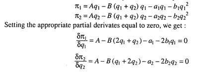
The basic behavioural assumption of the Cournot model is that each duopolist maximises his profit on the assumption that the quantity produced by his rival is invariant with respect to his own decision regarding output quantity. Duopolist I maximises π₁ with reference to q₁, treating q₂ as a parameter, and duopolist II maximises π₂, with reference to q₂, treating q₁ as a parameter. Setting the partial derivatives of (3) equal to zero, we get:

 

 

 

 

The first order (necessary) condition of profit-maximisation requires that each duopolist equates his marginal cost to his marginal revenue. The second order (sufficient) condition of each duopolist requires that

 

 

 

 

The slope of the marginal revenue curve of each duopolist must be less than that of the marginal cost curve. Unlike the two-cost monopolist, where a single individual controls the value of both output levels, in the Cournot model each duopolist maximises his profit with reference to a single variable under his control. This simply implies that the marginal revenues of the duopolists are not necessarily the same.

Let q = q₁ + q₂ and δq/δq₁ = δq/δq₂ = 1.

The marginal revenues of the duopolists are:

Since the demand curve is downward sloping the duopolist with the greater output will have the smaller marginal revenue (because a duopolist has to reduce price to sell more).

Equilibrium Condition:

The Cournot solution is simple enough. In this model, the duopolist market is in equilibrium if the values of q₁ and q₂ are such that each duopolist maximises his profit, taking the output of the sole rival as a parameter, and neither desires to change his output level. Thus, there is no conjectural variation in this model. The optimum solution (equilibrium condition) can be found out in this model by solving (3) for q₁ and q₂ if (4) is satisfied.

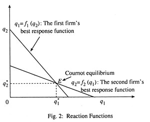
At this stage we have to introduce an additional step to get a more complete picture of duopoly. Reaction functions which express the output of each duopolist as a function of his rival’s output are determined by solving the first equation of (3) for q₁ and the second for q₂:

q₁ = f₁ (q₂)

q₂ = f₂ (q₁) … (6)

The reaction function of duopolist I gives a relationship between q₁ and q₂ with the property that, for any specified value of q₂, the corresponding value of q₁ maximises p₁. In a like man­ner, duopolist II’s reaction function gives the value of q₂ which maximises p₂ for any specified value of q₁. An equilibrium solution here is a pair of values for q₁ and q₂ which satisfy both reaction functions.

Let us suppose the demand and cost functions of duopolists are:

p = A – B (q₁ + q₂) C₁ = a₁q₁ + b₁q₁² ₂ = a₂q₂ + b₂q₂²

All parameters are positive here. So the profits of the duopolists are

The corresponding reaction functions are:

Since the parameters B, b₁q₁ and b₂, q₂ are all positive, an increase in output of ei­ther duopolist will lead to a fall in the other optimum (profit-maximising) output. The reaction functions are linear as shown in Fig. 2. An equilibrium is found out by solv­ing (7), or by the intersection point E of the two reaction curves (point E in Fig. 2).

The solution of (7) is

 

 

 

 

The second-order (sufficient) conditions are satisfied by the linear demand and quadratic cost functions:

 

 

Comments:

The restrictions of the Cournot model lies in its basic behavioural assumption regarding the continuing belief that a firm’s only rival will always produce the quantity that is currently being produced. Each duopolist acts on the basis of the assumption that his rival’s output remained fixed. However, this need not necessarily be true.

If we assume that equilib­rium is reached through a sequence of finite adjustments, one duopolist sets an output; this induces the other to adjust his output, which, in turn, induces the first to adjust his, and so on. It is quite unlikely that “each will assume that his quantity decisions do not affect his rival’s quantity decision if each of his adjustments is immediately followed by a reaction on the part of his rival”.

To be more specific, if equilibrium is assumed to be reached simultaneously, the optimal quantity of a duopolist is not given by q₁ =f₁(q₂), but by q₁ =f₁[f₂(q₁)] and, similarly for II, since each knows the behaviour pattern of his rival. Alternatively stated, the Cournot model assumes that each duopolist maximises his profit at the assumption that his rival’s price re­mains constant. But this is not a very realistic assumption for a homogeneous product. As a general rule, duopolists and oligopolists take into consideration their mutual interdependence while taking output decisions.

Extension:

The simple Cournot model can be extended to cover more than two firms. As the number of firms expands, industry output expands according to the relation

where n denotes the number of firms. Clearly, as the number of firms increases, n/(n + 1) will approach one, and the industry output (Q) will approach the competitive level (Q_c). In gen­eral, we can write the duopolists’ profit functions as π₁ (q₁, q₂) = q₁D (q₁ +q₂) – C (q₁) and π₂ (q₁, q₂) = q₂D (q₁ + q₂) – C (q₂) where D is the demand for, and C is the cost function. The first firm chooses a quantity q₁, where the partial derivatives of π, with functions to q₁ is equal to zero:

δπ₁ (q₁*, q₂)/δq₁ = 0

Of course, this is an implicit expression for the first firm’s best-response function because it determines the profit-maximising quantity of the first firm (q₁) for any value of q₂. Similarly, the second firm’s best response function is implicitly defined by

Δπ₂ (q₂*, q₁)/δq₂ = 0

The Cournot equation is then a pair of quantity q₁^C q₂^C that satisfies both the best-response functions.

Punishment Strategies:

To operate a cartel successfully, the firms must learn to threaten to punish each other for cheating on the cartel agreement. Let us consider a duopoly consisting of two identical firms such that each firm produces just half the monopoly amount of output where total profits will be maximised and each firm will get a payoff of π_p ( say).

In order to make this outcome stable, one firm threatens the other in terms of the production of output such that if any one of them tries to cheat by producing more than the joint industry profit level of output, then it will be punished by the other firms, who will be producing at the Cournot level of output forever. This is known as a punishment strategy.

Now we assume that cheating occurs, and the punishment is carried out. As the ultimate optimal response to Cournot behaviour is the Cournot behaviour, it will result in each firm receiving a per-period profit of, say π_c, such that

π_c < π_p

where π_c → Cournot payoff

π_p → Cartel payoff.

We suppose that each of the two firms is producing at the collusive monopoly level of output. If a firm produces more output, deviating from its quota of production, the level of its profit is such that

π_d > π_p

and it is the standard temptation facing a cartel member. Each firm has an incentive to capitalize on the high price by increasing its production, if each one restricts output and raises the price and for this there can be a punishment for cheating. Clearly, if a firm produces at the cartel amount, each one gets a steady flow of payments of π_p.

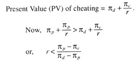
Thus, the present value of this flow today can be given by:

Present Value of cartel behaviour – π_p + π_p/r.

The firm gets a one-time benefit of profit, π_d, if it produces more than the cartel amount. This results is the reversion to Cournot behaviour:

Here the numerator of this fraction is positive, as the monopoly profits are larger than the Cournot profits, and the deviation is even more profitable than sticking with the monopoly quota which helps the denominator to be positive. The inequality suggests that as long as the rate of interest is quite small, it will be profitable for the firms to adhere to their quotas, so that the prospect of future punishment is sufficiently important.

2. The Bertrand Model:

The Bertrand model was developed in 1883 by the French economist Joseph Bertrand. Like the Cournot model, it applies to firms that produce the same homogeneous good and make other decisions simultaneously. This change may affect market outcome dramatically. The Bertrand model substitutes price π₁ and π₂ for quantities q₁ and q₂ as the variables to be chosen. Thus, the Cournot and Bertrand equilibrium are logical first cousins.

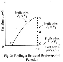
What is the first firm’s demand function if it takes its rivals’ price p₂ as given? The first firm will anticipate that if it charges a price higher than its rivals’ (p₁ > p₂), everyone will buy from its rival. If the first firm charges a lower price than its rivals’ (p₁ < p₂), however, everyone will buy from it. And if it charges a price equal to its rivals’ (p₁ = p₂), the firms will divide the market among them. The dia­gram for this profit function is shown in Fig. 3.

Here OM is the marginal cost of producing the commodity. The second firm’s price is p₂. The first firm’s profit function is composed of three segments. When p₁ < p₂, the first firm captures the entire mar­ket, and its profit increases as its price increases. When p₁ > p₂, the two firms split the total profits equal to distance CA, and each makes a profit equal to CB. When p₁ >p₂, the first firm’s profit is zero because it sells nothing when its price exceeds the second firm’s price.

Criticisms:

The Bertrand model has been criticised on two main grounds. First, when firms produce a homogeneous good, it is more natural to compete by setting quantities rather than prices. Second, even if firms do set prices and choose the same price (as the model predicts), what share of total sales will go to each one? The model assumes that sales would be divided equally among the firms, but there is no reason why this must be the case.

However, despite these shortcomings, the Bertrand model is useful because it shows how the equilibrium out­come in an oligopoly can depend crucially on the firms’ choice of strategic variable.

3. The Stackelberg Model:

The Stackelberg model (presented by the German economist Heinrich von Stackelberg) is a modified version of the Cournot model. In the Cournot model, we assume that two duopolists make their output decisions at the same time. The Stackelberg model examines what happens if one of the firms can set its output first. The Stackelberg model of duopoly is different from the Cournot model, in which neither firm has any opportunity to react.

The model is based on the assumption that the profit of each duopolist is a function of the output levels of both:

π₁ = g₁ (q₁, q₂) π₂ = g₂ (q₁, q₂) … (1)

The Cournot solution is found out by maximising π₁ with reference to q₁, assuming q₂ to be constant and π₂ with reference to q₂, assuming q₁ to be constant. In general, each firm might make some other assumption about the response (reaction) of its only rival. In such a situation, profit-maximisation by the two duopolists requires the fulfillment of the following two condi­tions:

 

 

 

 

The terms of δq₂ /δq₁ and δq₁/δq₂ represent what economists call the conjectural variation, i.e., the assumed response of each firm to the output of its lone rival. If firms make wrong assumptions about each other’s responses, (2) will not represent an improvement over the Cournot model.

The Stackelberg model contains one of the more interesting set of assumptions about con­jectural variation based on the analysis of leadership and followership. A follower obeys his reaction function q₁ =f₁ (q₂) or q₂ =f₂ (q₁) and adjusts his output level with a view to maximising his profits given the quantity decision of his rival, when he assumes to be a leader. But a leader does not obey his (the follower’s) reaction function. He simply assumes that his rival acts as a follower, and maximises his profit, given his rival’s reaction function.

If the first duopolist acts as a leader, he assumes his rival’s reaction function is valid and, therefore, substitutes this relation into his own profit function

π₁ = g₁[q₁, f(q₁)]

The first duopolist’s profit is now a function of q₁ alone. So it can be maximised with respect to this single variable. The second duopolist can also determine the maximum profit from leadership on the assumption that the first one obeys his reaction function and acts as a follower. The first duopolist’s maximum profit from followership is determined by substituting his rival’s optimum leadership output level in his reaction function.

Similarly, the second duopolists’ maximum profit from followership is determined by substituting the first duopolist’s optimum leadership output level in his reaction function. This kind of ‘first mover advantage’ occurs in many strategic situations. Each duopolist determines his maximum profit levels from both leadership and followership and seeks to play the role which yields the larger maximum.

Stackelberg thinks of four possible outcomes:

(1)1 desires to be a leader and 2 a follower;

(2) 2 desires to be a leader and 1 a follower;

(3) both desire to be leaders; and

(4) both desire to be the followers.

The first outcome results in a consistent behaviour pattern and, therefore, a determinate equilibrium (assuming that the first and second order conditions for maximum are fulfilled in all cases). Similarly, the second outcome results in a determinate equilibrium. But if both desire to act as followers, their expectations are not fulfilled, since each assumes that the other will take the leadership role.

Comparison with Cournot Model:

Even in terms of the Stackelberg model, the Cournot solution is achieved if each desires to act as a follower, knowing fully well that the other will also take a follower’s role. Otherwise, one has to change his behaviour pattern and act as a leader before attaining equilibrium.

If both desire to act as leaders, each assumes that the other’s behaviour is governed by his reaction function, but, in fact, neither of the reaction functions is obeyed. Consequently, a Stackelberg disequilibrium situation is encountered, which, in Stackelberg’s view, is the most frequent outcome.

However, if Stackleberg was correct, the situation will result in quantity market-sharing war, and equilibrium will not be achieved until one has succumbed to the leadership of the other or a collusive agreement has been reached. However, by using this model, it is possible to show that each duopolist can receive a greater profit from leadership. So it is quite obvious that both desire to act as leaders.

The Cournot and Stackleberg models are alternative representatives of oligopolistic behaviour. Which model is the more appropriate depends on the industry. In an industry where all firms are more or less identical, none of which has a pricing advantage or leadership position, the Cournot model is probably the more appropriate.

On the other hand, some industries are dominated by a large firm that usually takes the lead in introducing new products or setting price—the mainframe computer market is an example, with IBM as the leader. Then the Stackelberg model may be more realistic.

4. The Collusive Model:

Duopolists (or oligopolists) often recognise their mutual interdependence and agree to act to­gether (in collusion) in order to maximise the total profit of the industry. Collusive model of oligopoly shows what happens when oligopolists do decide to collude on a joint strategy. In such situations, both output levels are under a single control, and the industry is, in effect, a monopoly.

Let us suppose we represent total revenue as

R (q₁ + q₂) = R₁ (q₁, q₂) + R₂ (q₁, q₂) = (q₁ + q₂) F (q₁ + q₂)

Total profit is

π = π₁, + π₂ = R(q₁ +q₂) – C₁ (q₁) – C₂ (q₂)

This type of profit function is found in case of a two-plant monopolist. Here we substitute two plants by two producers. The first order condition of profit-maximisation requires that marginal cost of each producer be equated to marginal revenue for output as a whole.

In this model, the profit levels of two duopolists are determined as the basis of their indi­vidual profit functions. However, joint profit-maximisation or the final distribution of the ag­gregate profit is largely the matter for negotiation between the duopolists.

Like the Cournot equilibrium, the Bertrand equilibrium is individually rational, but collec­tively irrational. Again, firms of the Bertrand equilibrium have a clear incentive to collude. Does this mean that the collusive model makes better sense of oligopoly than do the Cournot and Bertrand models?

Not necessarily. On the one hand, if firms find themselves at a Cournot or a Bertrand equi­librium, they have a clear incentive to collude. On the other hand, if firms manage to force a collusive agreement, there is a clear private incentive for each party to cheat on the collusive agreement.

In the Cournot model, the individual incentive to cheat on a collusive agreement increases as the number of parties to the agreement increases, which means that the larger the number of firms in an industry, the less likely is a collusive equilibrium. If the number of firms is large enough, some firm or firms will succumb to the temptation to cheat, thereby destroying the collusive agreement.

The Market-sharing Solution:

Some economists have analysed the nature of oligopolistic interdependence in case of differen­tiated products. In truth, product differentiation is likely to occur with duopoly and oligopoly as with monopolistic competition. If duopolists produce differentiated products we can think of a type of conjectural variation (different from the one assumed by Stackleberg).

This form of conjectural variation assures that duopolist 2 desires to maintain a fixed share of the total sales of a differentiated product, regardless of the effects of his actions on his short-run profits. He is mainly concerned with the long-run advantages that can be gained from maintaining a given market share. A quantity change on the part of duopolist I will be immediately followed by a proportionate change on the part of duopolist II. The relation is:

 

 

where k is duopolist II’s market share, will always hold. Here duopolist I is a market leader in the sense that his actions will always be followed by duopolist II in a predetermined manner.

Duopolist I’s inverse demand function is p₁ = h₁ (q₁, q₂) and his profit function is p₁ = q₁h₁ (q₁, q₂) – C₁ (q₁).

Substituting from (1) for q₂,

 

 

Thus, duopolist I’s profit is a function of his own output (q₁) and may be maximised with reference to this single variable as long as duopolist II reacts to maintain his market share.

5. The Kinked Demand Curve Model:

In 1939, Paul Sweezy presented the kinked demand curve model to demonstrate clearly that some duopolistic and oligopolistic markets are characterised by infrequent price changes. Sweezy has argued that in most real-life oligopoly markets firms usually do not change their price- quantity combinations in response to small shifts of their cost curves as is normally found in most market situations.

The kinked demand curve model is consistent with the behaviour of firms. Starting from an initial price-quantity combination, if one of the duopolists lowers his price (increasing his quantity), the other is assumed to react by lowering his price (increasing his quantity) in order to maintain his market share. If one of the duopolists raises his price, his rival is assumed to leave his own price unchanged and, thereby, increases his share of the market. Price cuts are matched, but price increases are not.

Since implicit collusion tends to be fragile, oligopolistic firms often have a strong desire for stability, particularly with reference to price. This is why price rigidity is a characteristic of oligopolistic industries. Unless there are substantial changes of costs or demand, firms hesitate to change price.

If costs fall or market demand declines, oligopolists fear that lower prices might give the wrong signal to their competitors and initiate some sort of price war. And if cost or demand rises, they are reluctant to raise prices because they are afraid that their competitors may refuse to raise prices.

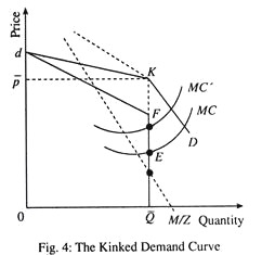
This price rigidity forms the basis of the kinked demand curve model of oligopoly. Accord­ing to this model, each firm faces a demand curve kinked at current prevailing price P̅, as shown in Fig. 4. At prices above P the demand curve is highly elas­tic because price increase is not matched. So the exist­ing firm will lose its market share considerably.

On the other hand, the firm believes that if it lowers its price below P̅, other firms will make matching price cuts, because they do not lose their market share. Thus, for price increase, the demand curve is inelastic. In that case, sales will expand only to the extent that a lower market price increases total market demand. Thus, nei­ther price cut, nor price increase is desirable. In each case, the firm loses.

Since the firm’s demand curve is kinked, its combined marginal revenue curve is discon­tinuous. This means that the firm’s cost can change without leading to price change. In this figure, marginal cost could increase but would still equal marginal revenue at the original out­put level. This means that price remains the same.

Comments:

The kinked demand curve model fails to explain oligopoly pricing. It says nothing about how marginal revenue firms arrived at the original price P̅ to start with. In fact, some arbitrary price is taken as both the starting and end point of our journey. Why firms did not arrive at some other price remains an open question. It just describes price rigidity but cannot explain it. In addition, the model has not been supported by empirical tests. In reality, rival firms do match price increases as well as price cuts.

Market-sharing Price Leadership:

Oligopolists often collude—jointly restrict supply to raise price and cooperate. This strategy can lead to higher profits. Collusion is, however, illegal. Moreover, one of the main impedi­ments to implicitly collusive pricing is the fact that it is difficult for firms to agree (without talking to each other) on what the price should be.

Coordination becomes particularly problem­atic when cost and demand conditions—and, thus, the ‘correct’ price—are changing. However, benefits of cooperation can be enjoyed without actually colluding. One way of doing this is through price leadership. Price leadership may be provided by a low-cost firm or a dominant firm.

In this context, we may draw a distinction between price signalling and price leadership. Price signalling is a form of implicit collusion that sometimes gets around this problem. For example, a firm might announce that it has raised its price with the expectation that its competi­tors will take this announcement as a signal that they should also raise prices. If competitors follow, all of the firms (at least, in the short run) will earn higher profits.

At times, a pattern is established whereby one firm regularly announces price changes and other firms in the industry follow. This type of strategic behaviour is called price leadership— one firm is implicitly recognised as the ‘leader’. The other firms, the ‘price followers’, match its prices. This behaviour solves the problem of coordinating price: Everyone simply charges what the leader is charging.

Price leadership helps to overcome oligopolistic firms’ reluctance to change prices—for fear of being undercut. With changes in cost and demand conditions, firms may find it increas­ingly necessary to change prices that have remained rigid for some time. In that case, they wait for the leader to signal when and by how much price should change.

Sometimes a large firm will naturally act as a leader; sometimes different firms will act as a leader from time to time. In this context, we may discuss the dominant Firm model of leadership. This is known as market- sharing price leadership.

6. The Dominant Firm Model:

In some oligopolistic markets, one large firm has a major share of total sales while a group of smaller firms meet the residual demand by supplying the remainder of the market. The large firm might then act as a dominant firm, setting a price that maximises its own profits.

The other firms, which individually could exert little, if any, influence over price, would then act as perfect competitors; they all take the price set by the dominant firm as given and produce accordingly. But what price should the dominant firm set? To maximise profit, it must take into account how the output of the other firms depends on the price it sets.

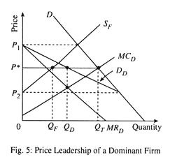
Fig. 5 shows how a dominant firm sets its prices. A dominant firm is one with a large share of total sales that sets price to maximise profits, taking into account the supply response of smaller firms. Here D is the market demand curve and S_F is the supply curve (i.e., the aggregate marginal cost curves of the smaller firms, called competitive fringe firms). The dominant firm must determine its demand curve D_D.

This curve is just the difference between market demand and the supply of fringe firms. For example, at price P₁, the supply of fringe firms is just equal to market demand. This means that the dominant firm can sell nothing at this price. At a price P₂ or less, fringe firms will not supply any of the good, in which case, the dominant firm faces the market demand curve. If price lies between P₁ and P₂, the dominant firm faces the demand curve D_D.

The marginal cost curve of the dominant firm corresponding to D_D is MR_D. The dominant firm’s marginal cost curve is MC_D. In order to maximise its profit, the dominant firm produces quantity Q_D at the interaction of MR_D and MC_D. From the demand curve D_D, we find P₀. At this price, fringe firms sell a quantity Q_F, thus the total quantity sold is Q_T = Q_D + Q_F.

7. Collusive Oligopoly: The Cartel Model:

Various models have been formulated to explain the strategic behaviour of firms in an oligopolistic market. A price (cut-throat) competition exists among the rivals who try to oust the others from the market. Sometimes there ex­ists a dominant firm that acts as the leader in the market while the others just follow the leader.

As a result, there happens to be a clear possibil­ity of the formation of a cartel by the rival firms in an oligopolistic market in order to eliminate competition among themselves. This is termed as “collusive oligopoly” because the firms some­how manage to combine together in order to be­have collectively as a single monopoly.

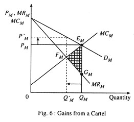
Now let us see graphically what incentives the firms get for forming a cartel. In Fig. 6, the market demand curve is given by the D_M the total supply curve is the horizontal summation of the marginal cost curves of all existing firms in the industry, which is denoted by MC_M.

The market equilibrium is attained at the point of intersection between the D_M (demand curve) and the marginal cost curve MC_M, if the firms compete with each other. OP_M is the equilibrium price at which the total output of the industry is OQ_M.

In order to determine its own quantity, each firm equates this price to its marginal cost. The sum of the quantities of the firms is OQ. If the firms form a cartel in order to act as a monopolist, the price rises to OP ‘_M and the quantity is reduced to OQ ‘_M to be in equilibrium. Now, when the quantity is being reduced by Q_MQ’_M, then all the firms together save the cost represented by the area below the MC_M curve which is Q_ME_MF_MQ ‘_M.

Thus, a rise in price due to a reduction in the quantity is followed by a decrease in the total revenue represented by the area below the MR_M curve, i.e., area Q_MG_MF_MQ’_M. This, in turn, shows that the cost saved exceeds the loss in revenue and, so, all the firms taken as a whole can increase their profit represented by the area E_MF_MG_M. The prospect of earning this extra profit actually acts as the incentive to form a cartel in the oligopoly market structure.

Since the cartel is formed, all firms agree together to produce the total quantity OQ’_M. In order to carry this out, each and every firm is allotted a quota or a certain portion of production such that the sum of all quotas is equal to OQ _M. For this, the best way of quota allotment would be to treat each firm as a separate entity (plant) under the same monopolist. Thus, all the firms have the same marginal cost (MC) such that MC = MR (marginal revenue).

Finally, the total profit is maximised because the total output is produced at the minimum cost.

Weakness:

Each and every firm can increase its profit by reducing the profits of other firms, simply by increasing its output quantity above the allotted quota. The system of cartel formation must guard against the desire of individual firms to violate the quota and the cartel breaks down when the cost of guarding against quota violation is very high.

The OPEC is an example of collusive oligopoly or cartel in which members (producers) explicitly agree to cooperate in setting prices and output levels. All the producers in an industry need not and often do not join the cartel. But if most producers adhere to the cartel’s agree­ments, and if market demand is sufficiently inelastic, the cartel may drive prices well above competitive levels.

Two conditions for success:

Two conditions must be fulfilled for cartel success. First, a stable cartel organisation must be formed whose members agree on price and production levels and both adhere to that agreement. The second condition is the potential for monopoly power. A cartel cannot raise price much if it faces a highly elastic demand curve. If the potential gains from cooperation are large, cartel members will have more incentive to share their organisa­tional problems.

Analysis of Cartel Pricing:

Cartel pricing can be analysed by using the dominant firm model of oligopoly. It is because a cartel usually accounts for only a portion of total production and must take into account the supply response of competitive (non-cartel) producers when it sets price. Here we illustrate the OPEC oil cartel.

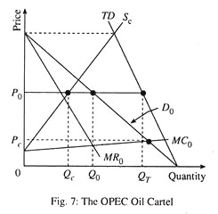
Fig. 7 illustrates the case of OPEC. Total demand TD is the world demand curve for crude oil, and S_c is the competitive (non-OPEC) supply curve. The demand for OPEC oil D₀ is the difference between total demand (TD) and competitive supply (SC), and MR₀ is the corresponding marginal revenue curve.

MC₀ is OPEC’s marginal cost curve; OPEC has much lower production costs than do non-OPEC producers. OPEC’s marginal revenue and marginal cost are equal at quantity Q₀, which is the quantity that OPEC will produce. Here we see from OPEC s demand curve that the price will be P₀.

Since both total demand and non-OPEC supply are inelastic, the demand for OPEC oil is also fairly inelastic; thus the cartel has substantial monopoly. In the 1970s, it used that power to drive prices well above competitive levels.

In this context, it is important to distinguish between short-run and long-run supply and demand curves. The total demand and non-OPEC supply curves in Fig. 7 apply to short-or intermediate-run analysis. In the long run, both demand and supply will be much more elastic, which means that OPEC’s demand curve will also be much more elastic.

We would thus expect that, in the long run, OPEC would be unable to maintain a price that is so much above the competitors’ level. In truth, during 1982-99, oil prices fell steadily, mainly because of the long- run adjustment of demand and non-OPEC supply.

However, cartel is not an unmixed blessing. No doubt cartel members can talk to one an­other in order to formalize an agreement. But it is not that easy to reach a consensus. Different members may have different costs, different assessments of market demand, and even different objectives, and they may, therefore, want to set prices at different levels.

Furthermore, each member of the cartel will be tempted to “cheat” by lowering its price slightly to capture a larger market share than it was allotted. Most often, only the threat of a long-term return to competi­tive prices deters cheating of this sort. But if the profits from cartelization are large enough, that threat may be sufficient.

---

Essay # 5. Sales (Revenue) Maximisation:

W.J. Baumol presented an alternative hypothesis to profit maximisation, viz., sales (revenue) maximisation. He has suggested that large oligopolistic firms do not maximise profit, but rather maximise sales revenue, subject to the constraint that profit equals or exceeds some minimum accepted level. Various empirical studies support Baumol’s hypothesis. And it accurately cap­tures some aspects of oligopolistic firms’ behaviour.

Most important, when firms are uncertain about their demand curve they actually face, or, when they cannot accurately estimate the marginal costs of their output (due to uncertainty about factor prices, or when they produce more than one product), the decision to try to maximise sales appears to be consistent with their long-term survival. This is why many oligopolist firms seek to maximise their market share in order to protect themselves from the adverse effects of uncertain market environment.

Graphical Analysis:

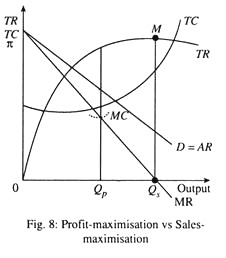
A revenue-maximising oligopolist would choose to produce that level of output for which MR = 0. When MR = 0, TR is maximum. That is, the oligopolist should proceed to the point at which selling any extra unit(s) actually leads to a fall in TR. This choice is illustrated in Fig. 8.

For the firm which faces the demand curve D, TR is maximum when output is q_s. For q < q_s, MR is positive. This means that selling more units increases TR (though not necessarily profit). For q > q_s, however, MR is negative. So further sales actually reduce TR because of price cuts that are necessary to induce consumers to buy more. We know that

MR = P(1 – 1/e_p) … (1)

MR = 0 if e_p = 1, in which case TR will be maximum. TR is constant in a small neighbourhood of that output quantity at M₁P = 0, TR is maximum, and when TR is maximum, e_p = 1.

We may now compare the revenue-maximisation choice with the profit-maximising level of output, q_s. At q_p, MR equals marginal cost MC in Fig. 8. Increasing output beyond q_p would reduce profits since MR < MC. Even though TR continues to increase up to q_s, units of output beyond q_p bring in less than they cost to produce. Since marginal revenue is positive at q_p, equation (1) shows that demand must be elastic (e_p> 1) at this point.

---

Essay # 6. Constrained Revenue Maximisation:

A firm that chooses to maximise TR is neither taking into account its costs nor the profitabil­ity of the output that it is selling. And it is quite possible that the output level q_s in Fig. 8 yields negative profit to the firm. However, it is not possible to any firm to survive for ever with negative profits. So it may be more realistic to assume that firms do meet some mini­mum level (target rate) of profit from their activities.

Thus, even though oligopolists may be prompted to produce more than q_p with a view to maximising revenue, they may produce less than q_p units in order to ensure an acceptable level of profit. They will, therefore, behave as constrained revenue maximises and will choose to produce an output level which lies between q_p and q_s.

Mathematical Analysis:

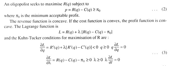
Let us assume that a unique unrestricted maximum profit π_m exists at the output q_p with R'(q_r) > 0, C”(q) > 0 for q> q_r, and R” (q) < 0 for q > 0. If π₀ > π_m, (2) cannot be satisfied and the maximum-revenue problem has no solution. A solution will exist if π₀ < π_m. If π₀ = π_m is q_r is the maximum solution since it is the only output that satisfies (2).

If π₀ < π_m, revenue will increase and profit will decrease as q is increased beyond q_r Thus, the oligopolist will continue to increase q until either (i) he reaches the unrestricted maximum of R(q); or (ii) (2) is satisfied as an equality, whichever occurs as the lower output. If (i), (3) states that R (q) = 0 and π = 0. If (ii) happens short of the output for (i), C'(q) > R'(q) > 0 and λ > 0. The multiplier π gives the rate at which revenue can be expanded per rupee of profit sacrificed.

An example will make the idea clear. Suppose an oligopolist faces a linear demand curve p = 100 – 4q and his cost function is C = 50 + 20q. Assume that Rs 334 = π₀ < π_m = Rs 350.

How much profit has to be sacrificed per unit of revenue?

The unrestricted maximum for R(q) is Rs 625 which occurs at q = 12.5 with π = Rs 325. This option may be excluded because it yields too low a profit. The equality of (2) is (100 – 4q²) – (50 + 20q) = Rs 334.

It may also be expressed as:

q² – 20q + 96 = 0.

The quadratic equation has the roots 8 and 12 with respective total revenues of Rs 544 and Rs 624. Thus, the revenue-maximising oligopolist produces 12 units which he sells at a price of Rs 52 to gain a total revenue of Rs 624 and a profit of Rs 334. By contrast, a profit-maximising oligopolist produces 10 units which he sells at a price of Rs 60 to gain a total revenue of Rs 600 and a profit of Rs 350. From (3), λ = 0.25. So the oligopolist sacrifices at the marginal rate of Rs 4 of profit to earn extra rupee of sales revenue.

---

Essay # 7. Game Theory:

The theories of duopoly and oligopoly lead to compact mathematical solutions with the cal­culus method. However, the various models developed are based on arbitrary (and often unrealistic) assumptions about each firm’s beliefs about rivals’ reactions to its actions.

The theory of games, developed by J. von Neumann and O. Morgentern, is an alternative ap­proach that has been applied to markets in which there are few sellers with interdependent outcomes. Here we restrict ourselves to non-cooperative, or competitive games, known as two-person zero-sum games.

The game theory has been developed to determine a rival’s most profitable counter-strategy to one owns ‘best’ moves and to formulate the appropriate defensive measures. A game is any situation in which players (the participants) make strategic decisions, i.e., decisions that take into account each one’s actions and responses, e.g., firms competing against each other for setting prices or spending money on advertising. Strategic decisions result in payoffs to the players: outcomes that generate rewards or benefits. For price-setting firms, the payoffs are profits.

Two-Person Zero-Sum Games:

A duopoly game consists of a single move on the part of each firm.

In this context, we define a few key terms:

Strategy:

A strategy is a rule or plan of action for playing the game; it is the specification of a particular move for one of the participants. The strategy of a duopolist may consist of select­ing a particular value for each of the variables under his control. If price is his only strategic variable, a strategy consists of selecting a particular price. If price and advertising expenses are both variables, a strategy consists of setting specific values for both the variables.

Each duopolist is assumed to have a large but a limited number of strategies, in which case there is no possibil­ity of continuous variation of the action variables. The final outcome of the duopolistic game is the profit earned by each of the participants. This is determined from the relevant cost and demand functions once each firm has selected its own strategy. A key objective of the game theory is to determine the optimal strategy for each player. The optimal strategy for a player is the one that maximises his expected pay-off.

Types of Games:

There are two criteria of classifying duopolistic games:

(i) The number of participants; and

(ii) The net outcome.

Since game theory is essentially a theory of deci­sion-making involving conflict the first criterion simply involves a counting of the number of participants with conflicting interests. Here we discuss any two-person games. The per­sons are like players of chess or card.

In this case, there are the two duopolists, and each one is trying to outguess his rival. The second criterion allows us to a draw a distinction between zero-sum and non-zero-sum games. A zero-sum game is one in which the sum of the out­comes—e.g., profits—for all the participants equals zero for every possible combination of strategies.

The economic games that firms play can be either cooperative or non-cooperative. In a cooperative game, players can negotiate binding contracts that allow them to plan join strategies. In a non-cooperative game, negotiation and enforcement of binding contracts are not possible.

In any game, however, the most important aspect of strategic decision-making is understanding one’s opponent’s point of view, and (assuming one’s opponent is rational), deducing his likely responses to actions. Two-person zero-sum games are competitive (non-cooperative) in nature. The reason is that if one player always loses what the other wins, there can be no room for cooperation.

---

Essay # 8. Payoff (Profit) Matrix:

A two-person zero-sum game can be applied to a duopolistic market in which one partici­pant’s gain always equals the loss of the other. In general, if I has m strategies and II has n strategies, the possible outcome of the game is given by the following payoff matrix which shows what I will receive as a result of each possible combination of strategy choice by himself and by II:

where the a_ij is I’s profit if I employs his ith strategy and II employs his jth. In case of zero-sum sum, the corresponding profit earned by II is – a_ij.

Maximin and Minimax Strategies:

Duopolists adopt two approaches, viz., maximin and minimax. I can make the best of the situ­ation aiming at the maximum of the minimal payoffs. This decision rule is called a maximin strategy.

Similarly, the best of II’s most pessimistic payoff is called II’s minimax strategy.

Let us consider the following payoff matrix:

If I employs his first strategy and II employs his second, I’s profit is 40, and II’s is – 40. If I employs his second strategy and II employs his third, I’s profit is – 10 and II’s is 10. The duopolist’s decision problem consists of choosing an optimal strategy. I desires the outcome (40) in the first row and second column of (2), and II desires the outcome (- 10) in the second row and third column. The final outcome depends upon the strategies of both duopolists, and neither has the power to enforce his desires.

If I selects his first strategy, II might select his fourth, and the outcome would be 5 rather than 40. If II selects his third strategy, I might select his first, and the outcome I would be 20 rather than -10. The theory of games postulates behav­iour patterns which allow the determination of equilibrium in these situations. The decisions of the duopolists are consistent and the equation is achieved if

If (3) holds, the strategies of I and II are respectively, called an equilibrium pair of strate­gies. In example (2), suppose I employs his first strategy. If II anticipates I’s choice, I’s profit will be 5. If I employed his second strategy, and II anticipated his choice, his profit would be -10. II will employ his fourth strategy and his loss will be limited to 5. Every other column of (2) has a maximum greater than 5. In this case,

The duopolists’ decisions are consistent, and an equilibrium is established. Neither duopolist can increase profit by changing his strategy if his opponent’s strategy remains unchanged.

Equilibrium (Saddle) Point:

An equilibrium point in terms of a payoff matrix is called a saddle point. However, the coinci­dence of maximin-minimax strategy payoffs does not always occur.

The Concept of Dominance:

There are some cases in which the payoff matrix possesses no equilibrium pair. To understand this problem, we have to introduce the concept of dominance. A dominant strategy is one that is optimal—no matter what an opponent does. In general, the ith row dominates the hth if a_ij ≥ a_hj for all j, and a_ij > a_hj for at least one j. A rational duopolist will never employ a dominant strategy. If he does, no equilibrium pair will exist.

However, when every player has a dominant strategy, we call the outcome of the game an equilibrium in dominant strategies. Equilibrium in dominant strategies refers to the outcome of a game in which each firm is doing the best it can, regardless of what its competitors are doing. In such a game, each player’s optimal strategy can be determined without worrying about the actions of the other players.

---