Derivation of Cost Schedules from a Production Function | Firm

In this article we will discuss how to derive cost schedules from a production function. Also learn about the relation between long-run average cost and marginal costs.

In economics the long run is not some date in the future. The long run simply means that all factors are variable to the firm. Therefore, one of the first decisions to be made by the owner and/or manager is the scale of operation, that is, the size of the firm. To make this decision the manager must know the cost of producing each relevant level of output. We may now examine how these long-run costs are determined.

Derivation of cost schedules from a production function:

Let us assume for analytical purposes that the firm’s level of usage of the inputs. Furthermore, assume that the production function has been evalu­ated for each level of output in the feasible range. The manager can derive an expansion path.

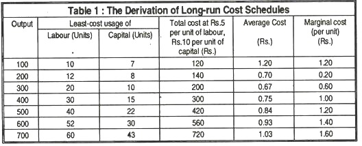
As an example, let us assume that the firm uses only two inputs, labour and capital, that cost Rs. 5 and Rs. 10 per unit, respectively. The charac­teristics of a derived expansion path are given in columns 2 and 3 of Table 1. Column 1 gives seven output levels and columns 2 and 3 give the optimal combinations of labour and capital for each output level, at the prevailing input prices. That is, these combinations make up seven points on the expansion path.

Column 4 shows the total cost of producing each level of output. For example, the least-cost method of producing 300 units of output requires 20 units of labour and 10 of capital. At Rs. 5 and Rs.10, respectively, the total cost is Rs.200. It should be emphasised that column 4 is a least-cost schedule for various rates of production. Obviously, the firm could pay more to produce any output; but it could not produce that output at a cost lower than the one given.

Average cost is shown in column 5. Average cost, the total cost of producing a given level of output divided by that output, is the number in column 4 divided by the corresponding number in column 1. Column 5 reflects an important assumed characteristic of long-run average cost — average cost first declines, reaches a minimum, then rises, as in the short run.

Long-run marginal cost, the change in total cost divided by the change in output, is provided in column 6. For example, increasing output from 100 to 200 units raises total cost from Rs.120 to Rs.140. Therefore, Rs.20 divided by the change in output, 100 units, gives a per-unit marginal cost of 20 paise. Note that marginal cost first decreases and then increases, as in the short run.

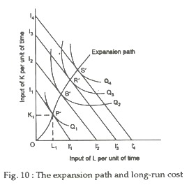
Let us now summarise the situation graphically. In Fig. 1 we continue to assume that out­put is produced using two in­puts, K and L. The known and fixed input prices give the con­stant input-price ratio, repre­sented by the slope of the isocost curves I₁I₁’, I₂I₂’ and so on.

Next, the known production function gives us the isoquant map, represented by isoquants Q₁, Q₂ and so forth in Fig. 10.

When all inputs are variable (that is, in the long run), the manager will choose input combinations that min­imise the cost of producing each level of output. In Fig. 10 these combina­tions give us the expansion path OP’B’R’S’. Given the factor-price ra­tio and the production function, the expansion path shows the combina­tions of inputs that enable the firm to produce each level of output at the least possible cost.

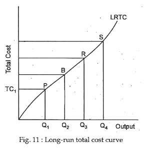
Now let us relate this expansion path to a long-run total cost (LRTC) curve. Fig. 11 shows graphically the “least-cost curve” associated with the expansion path in Figure 10. This least-cost curve is the long-run total cost curve. Points P, B, R and S associated with points P’, B’, R’ and S’ on the expansion path.

For example, in Fig.1 the least-cost combination of inputs that can produce Q₁ is K₁ units of capital and L₁ units of labour. Thus, in Figure 2 the lowest attainable cost of producing Q₁ units of output is TC₁, which is the price of capital times K₁ plus the price of labour times L₁. Every other point on LRTC is derived in the same way.

It is important to note that in the long run the firm may use different amounts and combinations of inputs to produce different levels of output. Nothing is fixed except the set of technological possibilities (the state of the art) and the prices at which the firm can purchase inputs.

Thus, completely different production processes may be used to achieve minimum cost at (say) Q₁ and Q₂ units of output. This “planning horizon” in which nothing is fixed except factor prices and technology is called the long run, and the associated curve that shows the minimum cost of producing each level of output is called the long-run total cost curve.

Definition:

A firm’s long-run total cost is the least cost at which each quantity of output can be produced when no input is fixed in quantity or rate of use.

The shape of the long-run total cost (LRTC) curve depends exclusively on the production function and the prevailing factor prices. The schedule in Table 1 and the curve in Fig. 11 reflect two of the commonly assumed characteristics of long-run total costs. Firstly, costs and output are directly related, that is the LRTC curve has a positive slope. It costs more to produce more, which is just another way of saying that resources are scarce or that one never gets something for nothing.

The second characteristic is that, costs first increase at a decreasing rate (until point B in Fig. 11), then increase at an increasing rate thereafter. This shape indicates that long-run marginal cost first decreases, then increases. We assume that all implicit costs of production are included in the LRTC curve. Since no costs are fixed in the long run, the long-run total cost curve begins at the origin rather than at some positive cost as is the case for the short-run total cost curve.

Long-run average and marginal costs:

We turn now to average and marginal cost in the long-run. Long-run average and marginal costs are defined just as they are in the short run.

Definitions:

Long-run average cost is the total cost of producing particu­lar output divided by that quantity.

LRAC = LRTC/Q

Long-run marginal cost is the addition to total cost attributable to an additional unit of output when all inputs are optimally adjusted.

LRMC = ∆LRTC/∆Q

It is, therefore, the change in total cost per unit of output as the firm moves along the long-run total cost curve (or the expansion path).

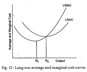
Fig. 12 illustrates typical long- run average and marginal cost curves. They have essentially the same shape as they have in the short run. Long-run average cost first declines, reaches a minimum (at Q₂ in Fig. 12), then increases. Long-run marginal cost first de­clines, reaches minimum at a lower output than that associated with minimum average cost (Q₁ in Fig. 12), and increases thereaf­ter.

The marginal cost curve crosses the average cost curve at the minimum of average cost (as it does in the short-run). The reasoning is the same as that given for short-run average cost, each additional unit produced adds less than average cost to total cost; so average cost must decrease.

When marginal cost is greater than average cost, each additional unit of the good produced adds more than average cost to total cost; so average cost must be increasing over this range of output. Thus, marginal cost must be equal to average cost when average cost is at its minimum.

We can summarise with the following:

1. LRTC rises continuously, first at a decreasing rate then at an increasing rate.

2. LRAC first declines, reaches a minimum, then rises. When LRAC is at its minimum, LRMC equals LRAC.

3. LRMC first declines, reaches a minimum and then increases. LRMC lies below LRAC over the range in which LRAC declines; it lies above LRAC when LRAC is rising.