Equilibrium of Firm and Industry: Definitions, Conditions and Difficulties

Equilibrium of Firm and Industry: Definitions, Conditions and Difficulties!

The word equilibrium has been taken from science. It is a state of no change where opposite forces become equal.

The consumer is in equilibrium when he is getting maximum satisfaction from his income.

Similarly, for an industry, equilibrium refers to a situation when there is no tendency for new firms to enter or exit. Now, the question arises, under what conditions such equilibrium situations will be achieved.

Equilibrium of Firm:

“A firm is a unit engaged in the production for sale at a profit and with the objective of maximizing profit.” -Watson

A firm is in equilibrium when it is satisfied with its existing level of output. The firm wills, in this situation produce the level of output which brings in greatest profit or smallest loss. When this situation is reached, the firm is said to be in equilibrium.

“Where profits are maximized, we say the firm is in equilibrium”. -Prof. RA. Bilas

“The individual firm will be in equilibrium with respect to output at the point of maximum net returns.” -Prof. Meyers

Conditions of the Equilibrium of Firm:

A firm is said to be in equilibrium when it satisfies the following conditions:

1. The first condition for the equilibrium of the firm is that its profit should be maximum.

2. Marginal cost should be equal to marginal revenue.

3. MC must cut MR from below.

The above conditions of the equilibrium of the firm can be examined in two ways:

1. Total Revenue and Total Cost Approach

2. Marginal Revenue and Marginal Cost Approach.

1. Total Revenue and Total Cost Approach:

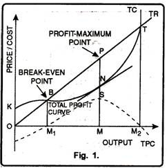
A firm is said to be in equilibrium when it maximizes its profit. It is the point when it has no tendency either to increase or contract its output. Now, profits are the difference between total revenue and total cost. So in order to be in equilibrium, the firm will attempt to maximize the difference between total revenue and total costs. It is clear from the figure that the largest profits which the firm could make will be earned when the vertical distance between the total cost and total revenue is greatest.

In fig. 1 output has been measured on X-axis while price/cost on Y-axis. TR is the total revenue curve. It is a straight line bisecting the origin at 45°. It signifies that price of the commodity is fixed. Such a situation exists only under perfect competition.

TC is the total cost curve. TPC is the total profit curve. Up to OM₁ level of output, TC curve lies above TR curve. It is the loss zone. At OM₁ output, the firm just covers costs TR=TC. Point B indicates zero profit. It is called the break-even point. Beyond OM₁ output, the difference between TR and TC is positive up to OM₂ level of output. The firm makes maximum profits at OM output because the vertical distance between TR and TC curves (PN) is maximum.

The tangent at point N on TC curve is parallel to the TR curve. The behaviour of total profits is shown by the dotted curve. Total profits are maximum at OM output. At OM₂ output TC is again equal to TR. Profits fall to zero. Losses are minimum at OM] output. The firm has crossed the loss zone and is about to enter the profit zone. It is signified by the break-even point-B.

2. Marginal Revenue and Marginal Cost Approach:

Joan Robinson used the tools of marginal revenue and marginal cost to demonstrate the equilibrium of the firm. According to this method, the profits of a firm can be estimated by calculating the marginal revenue and marginal cost at different levels of output. Marginal revenue is the difference made to total revenue by selling one unit of output. Similarly, marginal cost is the difference made to total cost by producing one unit of output. The profits of a firm will be maximum at that level of output whose marginal cost is equal to marginal revenue.

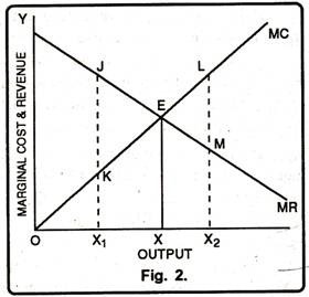
Thus, every firm will increase output till marginal revenue is greater than marginal cost. On the other hand, if marginal cost happens to be greater than marginal revenue the firm will sustain losses. Thus, it will be in the interest of the firm to contract the output. It can be shown with the help of a figure. In fig. 2 MC is the upward sloping marginal cost curve and MR is the downward sloping marginal revenue curve. Both these curves intersect each other at point E which determines the OX level of output. At OX level of output marginal revenue is just equal to marginal cost.

It means, firm will be maximizing its profits by producing OX output. Now, if the firm produces output less or more than OX, its profits will be less. For instance, at OX₁ its profits will be less because here MR = JX₁, while MC = KX₁ So, MR > MC. In the same fashion at OX₂ level of output marginal revenue is less than marginal cost. Therefore, beyond OX level of output extra units will add more to cost than to revenue and, thus, the firm will be incurring a loss on these extra units.

Besides first condition, the second order condition must also be satisfied, if we want to be in a stable equilibrium position. The second order condition requires that for a firm to be in equilibrium marginal cost curve must cut marginal revenue curve from below. If, at the point of equality, MC curve cuts the MR curve from above, then beyond the point of equality MC would be lower than MR and, therefore, it will be in the interest of the producer to expand output beyond this equality point. This can be made clear with the help of the figure.

In figure 3 output has been measured on X-axis while revenue on Y-axis. MC is the marginal cost curve. PP curve represents the average revenue as well as marginal revenue curve. It is clear from the figure that initially MC curve cuts the MR curve at point E₁. Point E₁ is called the ‘Break Even Point’ as MC curve intersects the MR curve from above. The profit maximizing output is OQ₁ because with this output marginal cost is equal to marginal revenue (E₂) and MC curve intersects the MR curve from below.

A. Determination of Short Run Equilibrium of Firm:

Short-run refers to that period in which fixed factors remaining unchanged the firms in order to incur maximum profits can vary their output by changing the variable factors like labour, raw material etc. In the short period, it is not necessary that the firms must earn super­normal or normal profits but even the firms may have to sustain the losses.

A firm may earn supernormal profits because in the short run, firms cannot enter the industry. Moreover, a firm may suffer losses, because in the short run, may not step up production even when price of the product falls. In case, it stops production temporarily, it will have to bear the loss of fixed cost which will constitute the minimum losses of the firm.

However, all the above stated possibilities have been explained as under:

(i) Supernormal Profits:

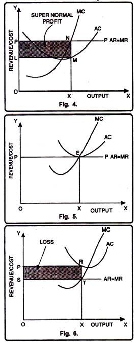
A firm is said to be in equilibrium when its marginal cost is equal to marginal revenue and marginal cost curve cuts the marginal revenue curve from below. A firm in equilibrium enjoys supernormal profits if average revenue exceeds marginal cost. This fact has been shown in fig 4.

In figure 4 outputs has been shown on horizontal axis and revenue on vertical axis. MC and AC are the marginal cost and average cost curves respectively. PP is the average revenue curve. It is clear from the figure that MC curve intersects the MR curve from below at point N which shows output OX. At this level of output price is NX and average cost is MX. Since average revenue is greater than average cost, the firm is earning super-normal profits MN per unit of output. Thus, the total super-normal profits of a firm will be equal to PLMN.

(ii) Normal Profit:

Normal profits refer to those profits where the average cost of the firm equals the average revenue. These profits cover just the reward for entrepreneurial services and are included in the cost of production. It can be shown with the help of a figure. In figure 5 the equilibrium has been depicted at point E. At point E marginal revenue is equal to marginal cost and marginal cost intersects the marginal revenue curve from below. The firm earns normal profits at OX output because at this output both the conditions of equilibrium are fulfilled.

(iii) Minimum Losses:

A firm in equilibrium incurs losses when it does not cover the average cost. In other words, when average revenue falls short of average cost, the firm has to sustain losses. In figure 6 the firm is said to be in equilibrium at point T. At this level of output both the conditions of equilibrium are satisfied i.e., marginal revenue is equal to marginal cost and marginal cost curve intersects the marginal revenue curve from below. Thus, it determines the OX level of output correspondingly price is OP. It means loss per unit of output is RT. Therefore, losses will be PSTR.

(iv) Shut Down Point:

Simple question is why firms continue producing the product if they are making losses. In the short run, the firms cannot go out of the industry by disposing off the plant. Why do they not shut down? It is because they cannot change the fixed factors and they have to face fixed costs even if the firm is shut down.

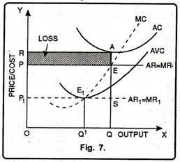
The firm can avoid only variable costs but it has to bear the fixed costs whether to produce or not. The firm will continue producing till the price covers the average variable cost. If the price covers some part of the average fixed costs besides the variable costs, the producer will continue producing. Thus the firm will continue producing so long as price exceeds average variable cost. The shut down point can be shown with the help of a diagram.

In diagram 7 equilibrium is at E where MR = MC and MC cuts MR from below. The price is EQ and OQ is the output. This price covers the average variable cost. Average cost corresponding to this output is AQ. In that way loss per unit is AE which is equal to average fixed cost. The total losses are equal to total fixed costs. If price is slightly below OP, level, the firm will not produce at all. The firm will simply shut down production and wait for some good days to come.

Shut Down Point (Losses=Total Fixed Costs):

However, the firm may continue to operate even under such a situation because of the following reasons:

1. The firm may continue to operate because a higher valuation (value) is given to an on­going concerns rather than a closed down firm.

2. More prestige is attached to the owner or manager of a on-going concern than to that of a firm that has closed down or ceased to operate.

3. By keeping the operation going, the firm will not lose competent personnel.

4. The firm may continue to operate in the hope of earning profits in future.

B. Determination of Long Run Equilibrium of the Firm:

Long run refers to that period in which the producer can change its supply by changing all the factors of production. In other words, the producer has the sufficient time to adjust their supplies according to the changed demand conditions.

Moreover, new firms can also enter and existing firms can leave the industry. In the long-run, the firm is said to be in equilibrium when marginal cost is equal to price. Besides it, the firm under perfect competition to be in equilibrium-price must be equal to average cost. Generally, in the long run, firm in equilibrium earns normal profits. If the firms happen to earn the super normal profits in the long period, the existing firms will increase their production.

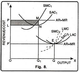
Lured by super normal profits some new firms will enter into the industry. The total supply of the product will increase and the price falls down. Thus, due to fall in price the firms will get normal profits. In case price of the product is less than the average cost, the firms would make losses. These losses would induce some firms to leave the industry. Consequently the output of the industry will fall which will raise the price, hence, the firms will begin to earn normal profits. It can be shown with the help of a figure 8.

In figure 8 output has been depicted on X-axis while revenue on Y-axis. SAC is the short run average cost curve and LAC is the long run average cost curve. Similarly, SMC and LMC are the short run marginal cost and long run marginal cost curves respectively.

Let us suppose that the industry determines OP price. At this price firms are producing with SAC₁ and is earning super normal profits equal to the shaded area PLNM. Lured by these super normal profits, the existing firms will increase their production capacity, thus, the new firms will enter the industry. As a result of the entry of the new firms supply of the product will increase which will lead to a fall in price.

Thus, the price will fall to OP’. At this price, the firm will be in equilibrium at point E and will produce OQ level of output. It is due to the reason that at point E, marginal revenue, long run marginal cost, average revenue and long run average cost are all equal and the firm earns normal profits.

Symbolically:

MR = LMC = AR = LAC = SAC = SMC = Price

Difficulties of TR-TC Approach:

The main difficulties of TR and TC approach are as under:

1. It is very difficult to analyze at what level of output profits are maximum.

2. It is difficult to see at a glance the maximum vertical distance between TR and TC approach.

3. It is very difficult to discover the price per unit of output.

Equilibrium of Industry:

The group of firms producing homogeneous product is called industry. In fact the concept of industry exists only under perfect competition. An industry is said to be in equilibrium when it has no tendency to increase or decrease its level of output.

According to Prof. Hansen, “An industry will be in equilibrium when there is no tendency for the size of the industry to change i.e., when no firms wish to leave it and no new firms are being attracted to it.” New firms will have no tendency to enter the industry when existing firms are enjoying normal profits. The normal profits earned by a firm are included in total cost.

In this way equilibrium for the industry means that firms are neither moving in or nor moving out. It means that the level of profits in it is neither above nor below the normal level and hence is equal to it.

Conditions of Equilibrium of an Industry:

1. Constant Number of Firms:

An industry will be in equilibrium when the number of firms remains constant. In this situation, no new firms will enter and no old firms will leave the industry.

2. Equilibrium of Firms:

An industry will be in equilibrium when all firms operating in it are in equilibrium and have no tendency to increase or decrease the level of output.

(i) Short Run Equilibrium of Industry:

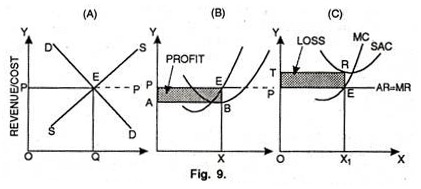
In the short run, the industry is said to be in Equilibrium when all the firms operating under it are in equilibrium. But for the industry to be in full equilibrium in the short run is very rare. Full equilibrium position is possible when firms earn normal profits. In the short run firms can also earn supernormal profits or incur losses. It can be shown with the help of fig. 9.

In fig. 9 (A) DD is the industry’s demand curve and SS represents the supply curve. Both these curves intersect each other at point E which establishes equilibrium of the industry. At this equilibrium point, industry sets price OP and produces OQ level of output. But, it will not be the full equilibrium of the industry.

In fig. B the firms are enjoying supernormal profits as indicated by ABED. In fig. 9 C, the firms are incurring losses equal to the shaded area PERT. In the long run, firms incurring losses will leave the industry. On the other hand, firms getting supernormal profits will expand their production capacity. Lured by supernormal profits new firms will enter the industry. Consequently, industry will be in equilibrium in the short run only if all firms are enjoying normal profits.

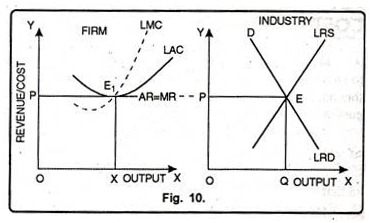
(ii) Long Run Equilibrium of the Industry:

The long run equilibrium of the industry can be shown with the help of a figure 10. In the long run the industry will be in equilibrium at a point where long run supply (LRS) is equal to long run demand (LRD). This determination of price is OP and output OQ. The firm will follow this price and will be in equilibrium at E₁. Here, the firms will earn just normal profits. Thus, according to Left-witch, “The existence of long run industry equilibrium requires long run individual equilibrium at no profit no loss level of operation”.