A. Interdependence in the Economy:
We have adopted a partial equilibrium approach, concentrating on decisions in a particular segment of the economy in isolation of what was happening in other segments, under the ceteris paribus assumption.
We examined the utility-maximizing behaviour of a household under the assumption that its income was given, although income depends on the amount of labour and other factors of production that the consumer owns and on their prices (wage, rental of capital, etc.).
The ceteris paribus assumption was useful in that it enabled us to study the individual’s demand for different commodities in isolation from influences arising from other parts of the economy.
ADVERTISEMENTS:
We studied the production decision of a firm on the assumption that factor prices, the state of technology and the prices of commodities were given. The ceteris paribus assumption allowed us to study the cost-minimization behaviour of a firm in isolation from such factors as the demands for the products, which in turn are influenced by the level of employment, income and tastes of consumers.
Product markets, where buyers and sellers interacted with each other and among themselves to determine prices and levels of outputs of various commodities, were studied under the ceteris paribus assumption; relationships with other markets were ignored.
Factor markets, where firms and households as owners of productive resources interacted with each other and among themselves to determine prices and quantities of various factors employed, were also analysed on the basis of the ceteris paribus assumption. The interrelationship between the various factor markets and commodity markets were left out of the analysis. In summary, the basic characteristic of a partial equilibrium approach is the determination of the price and quantity in each market by demand and supply curves drawn on the ceteris paribus clause. Each market in the Marshallian methodology is regarded independently of the others.
However, a fundamental feature of any economic system is the interdependence among its constituent parts. The markets of all commodities and all productive factors are interrelated, and the prices in all markets are simultaneously determined. For example, consumers’ demands for various goods and services depend on their tastes and incomes.
ADVERTISEMENTS:
→ In turn, consumers’ incomes depend on the amounts of resources they own and factor prices.
→ Factor prices depend on the demand and supply of the various inputs.
→ The demand for factors by firms depends not only on the state of technology but also on the demands for the final goods they produce.
→ The demands for these goods depend on consumers’ incomes, which, as we saw, depend on the demand for the factors of production.
ADVERTISEMENTS:
This circular interdependence of the activity within an economic system can be illustrated with a simple economy composed of two sectors, a consumer sector, which includes households and a business sector, which includes firms.
It is assumed that:
(a) All production takes place in the business sector;
(b) All factors of production are owned by the households;
(c) All factors are fully employed;
(d) All incomes are spent.
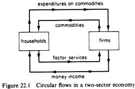
The economic activity in the system takes the form of two flows between the consumer sector and the business sector: a real flow and a monetary flow (figure 22.1).
The real flow is the exchange of goods for the services of factors of production: firms produce and offer final goods to the household sector, and consumers offer to firms the services of factors which they own. The monetary flow is the real flow expressed in monetary terms. The consumers receive income payments from the firms for offering their factor services. These incomes are spent by consumers for the acquisition of the finished goods produced by the business sector.
ADVERTISEMENTS:
The expenditures of firms become the money incomes of the households. Similarly, the expenditures of households become the receipts of firms, which they once again pay the households for the factor services which they supply.
The real flow and the monetary flow, which represent the transactions and the interdependence of the two sectors, move in opposite directions. They are linked by the prices of goods and factor services. The economic system is in equilibrium when a set of prices is attained at which the magnitude of the income flow from firms to households is equal to the magnitude of the money expenditure flow from households to firms.
The interdependence of markets is concealed by the partial equilibrium approach. Markets consist of buyers and sellers. Thus an economic system consists of millions of economic decision-making units who are motivated by self-interest. Each one pursues his own goal and strives for his own equilibrium independently of the others. In traditional economic theory the goal of a decision-making agent, consumer or producer, is maximisation of something.
The consumer maximises satisfaction subject to a budget constraint. The firm maximizes profit, subject to the technological constraint of the production function. A worker determines his supply of labour by maximising satisfaction derived from work-leisure opportunities, subject to a given wage rate. The problem is to determine whether the independent, self-interest motivated behaviour of economic decision-makers is consistent with each individual agent’s attaining equilibrium. All economic units, whether consumers, producers, or suppliers of factors, are interdependent.
ADVERTISEMENTS:
General equilibrium theory deals with the problem of whether the independent action by each decision-maker leads to a position in which equilibrium is reached by all. A general equilibrium is defined as a state in which all markets and all decision-making units are in simultaneous equilibrium. A general equilibrium exists if each market is cleared at a positive price, with each consumer maximising satisfaction and each firm maximising profit.
The scope of general equilibrium analysis is the examination of how this state can, if ever, be reached, that is, how prices are determined simultaneously in all markets, so that there is neither excess demand nor excess supply, while at the same time the individual economic units attain their own goals.
The interdependence between individuals and markets requires that equilibrium for all product and factor markets as well as for all participants in each market must be determined simultaneously in order to secure a consistent set of prices. General equilibrium emerges from the solution of a simultaneous equation model, of millions of equations in millions of unknowns.
The unknowns are the prices of all factors and all commodities and the quantities purchased and sold (of factors and commodities) by each consumer and each producer. The equations of the system are derived from the maximising behaviour of consumers and producers, and are of two types: behavioural equations describing the demand and supply functions in all markets by all individuals, and clearing-the-market equations.
ADVERTISEMENTS:
In principle a simultaneous-equation system has a solution if the number of independent equations is equal to the number of unknowns in the system. This approach has been followed by the founder of general equilibrium analysis Leon Walras.
B. The Walrasian System:
The most ambitious general equilibrium model was developed by the French economist Leon Walras (1834-1910). In his Elements of Pure Economics Walras argued that all prices and quantities in all markets are determined simultaneously through their interaction with one another. Walras used a system of simultaneous equations to describe the interaction of individual sellers and buyers in all markets, and he maintained that all the relevant magnitudes (prices and quantities of all commodities and all factor services) can be determined simultaneously by the solution of this system.
In the Walrasian model the behaviour of each individual decision-maker is presented by a set of equations. For example, each consumer has a double role: he buys commodities and sells services of factors to firms. Thus for each consumer we have a set of equations consisting of two subsets: one describing his demands of the different commodities, and the other his supplies of factor inputs.
Similarly, the behaviour of each firm is presented by a set of equations with two subsets one for the quantities of commodities that it produces, and the other for the demand for factor inputs for each commodity produced. The important characteristic of these equations is their simultaneity or interdependence. The solution of this system of millions of simultaneous equations defines the ‘unknowns’ of the model, namely the prices and quantities of all commodities and all factor inputs.
In a general equilibrium system of the Walrasian type there are as many markets as there are commodities and factors of production. For each market there are three types of functions demand functions, supply functions and a ‘clearing-the-market’ equation, which stipulates that the quantities demanded be equal to the quantities supplied. In a commodity market the number of demand functions is equal to the number of consumers, and the number of the supply functions is equal to the number of firms which produce the commodity.
ADVERTISEMENTS:
In each factor market the number of demand functions is equal to the number of firms multiplied by the number of commodities they produce. The number of supply functions is equal to the number of consumers who own (ex hypothesis) the factors of production.
A necessary (but not sufficient) condition for the existence of a general equilibrium is that there must be in the system as many independent equations as the number of unknowns. Thus the first task (in establishing the existence of a general equilibrium) is to describe the economy by means of a system of equations, defining how many equations are required to complete (and solve) the system.
For example, assume that an economy consists of two consumers, A and B, who own two factors of production, K and L These factors are used by two firms to produce two commodities, X and Y. It is assumed that each firm produces one commodity, and each consumer buys some quantity of both. It is also assumed that both consumers own some quantity of both factors (but the distribution of ownership of factors is exogenously determined).
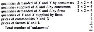
In this simple model we have the following ‘unknowns’:
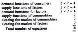
To find these unknowns we have the following number of equations:
Since the number of equations is equal to the number of unknowns, one should think that a general equilibrium solution exists. Unfortunately, the equality of numbers of equations and unknowns is neither a sufficient nor a necessary condition for the existence of a solution. In the Walrasian system one of the equations is not independent of the others there is a ‘redundant equation’ in the system which deprives the system of a solution, since the number of unknowns is larger than the number of independent equations. In this model the absolute level of prices cannot be determined.
General equilibrium theorists have adopted the device of choosing arbitrarily the price of one commodity as a numeraire (or unit of account) and express all other prices in terms of the price of the numeraire. With this device prices are determined only as ratios: each price is given relative to the price of the numeraire. If we assign unity to the price of the numeraire, we attain equality of the number of simultaneous equations and unknown variables (the number of unknowns is reduced to 17 in our example).
However, the absolute prices are still not determined: they are simply expressed in terms of the numeraire. This indeterminacy can be eliminated by the introduction explicitly in the model of a money market, in which money is not only the numeraire, but also the medium of exchange and store of wealth.
Even if there is equality of independent equations and unknowns, there is no guarantee that a general equilibrium solution exists. The proof of the existence of a general equilibrium solution is difficult. Leon Walras was never able to prove the existence of a general equilibrium.
In 1954 Arrow and Debreu provided a proof of the existence of a general equilibrium in perfectly competitive markets, in which there are no indivisibilities and no increasing returns to scale. Furthermore, in 1971 Arrow and Hahn proved the existence of a general equilibrium for an economy with limited increasing returns and monopolistic competition, without indivisibilities. Both proofs are limited to specific market structures and are based on restrictive assumptions, regarding in particular the necessity of ‘well-behaved’ continuous production and demand functions.
Thus the available ‘existence proofs’ do not hold for the typical real world cases of discontinuities and indivisibilities in production processes. Our current state of knowledge does not enable us to be sure of the existence of a general equilibrium in the real world, which is dominated by oligopolistic firms and production processes which are characterised by indivisibilities.
ADVERTISEMENTS:
However, the proof of the existence of general equilibrium for a perfectly competitive economy (with no indivisibilities and no increasing returns to scale) is very important, because a perfectly competitive system has certain ideal properties: it results in an efficientallocation of resources.
Apart from the existence problem, two other problems are associated with an equilibrium: the problem of its stability and the problem of its uniqueness.
C. Existence, Uniqueness and Stability of an Equilibrium:
Three problems arise in connection with a general equilibrium:
1. Does a general equilibrium solution exist? (Existence problem.)
2. If an equilibrium solution exists, is it unique? (Uniqueness problem.)
ADVERTISEMENTS:
3. If an equilibrium solution exists, is it stable? (Stability problem.)
These problems can best be illustrated with the partial-equilibrium example of a demand-supply model. Assume that a commodity is sold in a perfectly competitive market, so that from the utility-maximising behaviour of individual consumers there is a market demand function, and from the profit-maximising behaviour of firms there is a market supply function. An equilibrium exists when at a certain positive price the quantity demanded is equal to the quantity supplied.
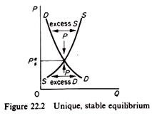
The price at which Qd = Qs is the equilibrium price. At such a price there is neither excess demand nor excess supply. (The latter is often called negative excess demand.) Thus an equilibrium price can be defined as the price at which the excess demand is zero the market is cleared and there is no excess demand.
The equilibrium is stable if the demand function cuts the supply function from above. In this case an excess demand drives price up, while an excess supply (excess negative demand) drives the price down (figure 22.2).
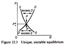
The equilibrium is unstable if the demand function cuts the supply function from below. In this case an excess demand drives the price down, and an excess supply drives the price up (figure 22.3).
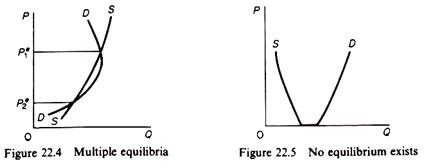
In figure 22.4 we depict the case of multiple equilibria. It is obvious that at Pe1 there is a stable equilibrium, while at Pe2 the equilibrium is unstable. Finally in figure 22.5 an equilibrium (at a positive price) does not exist.
It should be clear from the above discussion that (a) the existence of equilibrium is related to the problem of whether the consumers’ and producers’ behaviour ensures that the demand and supply curves intersect (at a positive price); (b) the stability of equilibrium depends on the relationship between the slopes of the demand and supply curves; (c) the uniqueness of equilibrium is related to the slope of the excess demand function, that is, the curve which shows the difference between QD and Qs at any one price. In fact the three basic questions related to the existence, stability and uniqueness of an equilibrium can be expressed in terms of the excess demand function.
E(Pi ) = QD(Pi) — Qs(Pi)
To see this we redraw below figures 22.2-22.5 in terms of the excess demand function. For each of these cases we have derived the relevant excess demand function by subtracting Qs from QD at all prices.
From the redrawn diagrams (in conjunction with the corresponding ones 22.2-22.5) we can draw the following conclusions:
1. The excess demand function, E{P), intersects the vertical (price)-axis when there is an equilibrium, that is, when the excess demand is zero. If QD = Qs, then E(P) = 0.
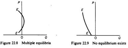
2. There are as many equilibria as the number of times that the excess demand curve E(P) intersects the vertical price-axis (figure 22.8).
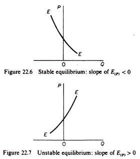
3. The equilibrium is stable if the slope of the excess demand curve is negative at the point of its intersection with the price-axis (figure 22.6).
4. The equilibrium is unstable if the slope of the excess demand curve is positive at the point of its intersection with the price-axis (figure 22.7).
5. If the excess demand function does not intersect the vertical axis at any one price, an equilibrium does not exist (figure 22.9).
The above analysis of the existence, stability and uniqueness in terms of excess demand functions can be extended to general equilibrium analysis.
D. A Graphical Treatment Of The Two-Factor, Two-Commodity, Two-Consumer (2 X 2 X 2) General Equilibrium Model:
Now we use graphical analysis to show the general equilibrium of a simple economy in which there are two factors of production, two commodities (each produced by a firm) and two consumers. This is known as the 2 x 2 x 2 general equilibrium model. We will restrict our analysis to the perfectly competitive market system, since with free competition it has been proved that a general equilibrium solution exists (given some additional assumptions about the form of the production and demand functions). Furthermore we will be concerned with the static properties of general equilibrium and not with the dynamic process of reaching the state of such an equilibrium, the latter having been sketched in the preceding section.
Assumptions of the 2 X 2 X 2 Model:
1. There are two factors of production, labour (L) and capital (K), whose quantities are given exogenously. These factors are homogeneous and perfectly divisible.
2. Only two commodities are produced, X and Y. Technology is given. The production functions of the two commodities are represented by two isoquant maps, with the usual properties. The isoquants are smooth and convex to the origin, implying diminishing marginal rate of factor (technical) substitution along any isoquant. Each production function exhibits constant returns to scale. Finally, it is assumed that the two production functions are independent: there are no external economies or diseconomies for the production activity of one product arising from the production of the other.
3. There are two consumers in the economy, A and B, whose preferences are represented by ordinal indifference curves, which are convex to the origin, exhibiting diminishing marginal rate of substitution between the two commodities. It is assumed that consumer choices are independent: the consumption patterns of A do not affect B’s utility, and vice versa. Bandwagon, snob, Veblenesque and other ‘external’ effects are ruled out. Finally, it is assumed that the consumers are sovereign, in the sense that their choice is not influenced by advertising or other activities of the firms.
4. The goal of each consumer is the maximisation of his own satisfaction (utility), subject to his income constraint.
5. The goal of each firm is profit maximisation, subject to the technological constraint of the production function.
6. The factors of production are owned by the consumers.
7. There is full employment of the factors of production, and all incomes received by their owners (A and B) are spent.
8. There is perfect competition in the commodity and factor markets. Consumers and firms pursue their goals faced by the same set of prices (Px, Py, w, r).
In this model a general equilibrium is reached when the four markets (two commodity markets and two factor markets) are cleared at a set of equilibrium prices (Px, Py, w, r) and each participant economic agent (two firms and two consumers) is simultaneously in equilibrium.
The general equilibrium solution thus requires the determination of the values of the following variables:
The total quantities of the two commodities X and Y, which will be produced by firms and bought by the consumers.
The allocation of the given K and L to the production of each commodity (Kx, Ky, Lx, Ly).
The quantities of X and Y which will be bought by the two consumers (XA, XB, YA, YB).
The prices of commodities (Px and Py) and of the factors of production (wage w, and rental of capital r).
The distribution of factor ownership between the two consumers (KA, KB, LA, LB). The quantities of factors multiplied by their prices define the income distribution between A and B, and hence their budget constraint.
General equilibrium and the allocation of resources:
In figure 22.26 the general equilibrium solution is shown by points T (on the production possibility curve) and T (on the Edgeworth contract curve). These points define six of the ‘unknowns’ of the system, namely the quantities to be produced of the two commodities (Xe and Ye), and their distribution among the two consumers (XAe, XBe, YAe, YBe). We examine the determination of the allocation of resources between X and Y. The determination of the remaining unknowns (prices of factors and commodities, and the distribution of income between the two consumers) is examined in two separate sections below.
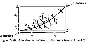
Point T on the production transformation curve (figure 22.26) defines the equilibrium product mix Ye and Xe. Recalling that the PPC is the locus of points of the Edgeworth contract curve of production mapped on the product space, point T corresponds to a given point on this contract curve, say T” in figure 22.28.
Thus T” defines the allocation of the given resource endowments in the production of the general equilibrium commodity mix. The production of Xe absorbs Lx of labour and Kx of capital, while Ye employs the remaining quantities of factors of production; Ly and Ky. Thus four more ‘unknowns’ have been defined from the general equilibrium solution.
Prices of commodities and factors:
The next step in our analysis is to show the determination of prices in the general equilibrium model, under perfect competition.
In the simple 2 x 2 x 2 model there are four prices to be determined, two commodity prices, Px and Py, and two factor prices, the wage rate w, and the rental of capital r. We thus need four independent equations. However, given the assumptions of the simple model, we can derive only three independent relations.
1. Profit maximisation by the individual firm implies least-cost production of the profit-maximising output. This requires that the producer adjusts his factor mix until the MRTS of labour for capital equals the w/r ratio
MRTSxL,k = w/r = MRTSyL,K (5)
In other words the individual producer maximises his profit at points of tangency between the isoquants and isocost lines whose slope equals the factor price ratio.
2. In perfect factor and output markets the individual profit-maximising producer will employ each factor up to the point where its marginal physical product times the price of the output it produces just equals the price of the factor
w = (MPPL,X).(PX) = (MPPL,y).(Py) (6)
r = (MPPK,x) . (Px) = (MPPk,y) . (Py) (7)
3. The individual consumer maximises his utility by purchasing the output mix which puts him on the highest indifference curve, given his income constraint. In other words maximisation of utility if attained when the budget line, whose slope is equal to the ratio of commodity prices Px/Py, is tangent to the highest utility curve, whose slope is the marginal rate of substitution of the two commodities
MRSAy,X = Py/Px = MRSBy,x (8)
Although we have four relations between the four prices, one of them is not independent. Because, dividing (6) and (7), we obtain
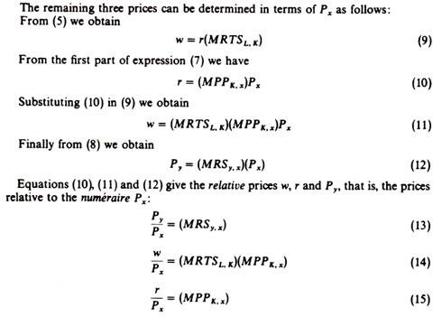
Which is the same as expression (5). Thus we have three independent equations in four unknowns. Apparently the absolute values of w, r, Px and Py are not uniquely determined (although the general equilibrium solution is unique). Prices in the Walrasian system are determined only up to a ratio or a scale factor. We can express any three prices in terms of the fourth, which we choose arbitrarily as a numeraire or unit of account. For example assume that we choose Px as the numeraire.
The terms in brackets are known values, that is, values determined by the general equilibrium solution and the maximising behaviour of economic decision-makers with a given state of technology and given tastes.
Note that any good can serve as numeraire, and the change of numeraire leaves the relative prices unaffected. We can also assign any numerical value to the price of the numeraire. For convenience Px is assigned the value of 1. But if, for example, we choose to set Px = £b, then the price of y in £ will be
Py = b. Py /Px (pounds)
This, however, does not mean that the absolute level of the prices of the system is determined. It simply illustrates the fact that we can assign to the price of the numeraire any value we choose.
The reason that the prices are determined only up to a ratio is that money has not been introduced in the system as a commodity used for transactions or as a store of
wealth. In a system with perfect certainty, where, for example, nobody would think of holding money, only relative prices matter. The three equations (13)—(15) establish the price ratios implied by the unique general equilibrium solution, and the absolute values of prices are of no importance.
However, the general equilibrium model can be completed by adding one (or more) monetary equation. Then the absolute values of the four prices can be determined. Unless a market for money is explicitly introduced, the price side of the model depends on an endogenous numeraire.
Factor ownership and income distribution:
For the simultaneous equilibrium of production and consumption, consumers must earn the ‘appropriate’ incomes in order to be able to buy the quantities of the two commodities (XA, XB, YA, YB) implied by point T in figure 22.26.
Consumers’ income depends on the distribution of factor ownership (quantities of factors which they own) and on factor prices. We saw in the preceding paragraph that the prices of factors are determined only up to a ratio. This, however, is adequate for the required income distribution, if the ownership of factors by A and B is determined. For this purpose we require four independent relations, given that we have four unknowns (KA, KB, LA, LB).
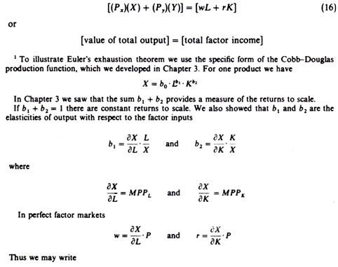
From the assumption of constant returns to scale we can make use of Euler’s ‘product exhaustion theorem’. This postulates that, with constant returns to scale, the total factor income is equal to the total value of the product of the economy (in perfect factor markets, where inputs are paid their marginal product)
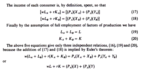
Thus we have three independent equations in four unknowns (KA, KB, LA, LB), whose values cannot be uniquely determined. The general equilibrium solution does not give absolute values for the distribution of ownership of the factors and money incomes between consumers A and B.
This indeterminacy can be resolved only partly if one fixes arbitrarily the value of one of the four factor endowments, and then allocate the remaining three so as to make the individual incomes of A and B such as to lead them willingly to the consumption pattern implied by point T in figure 22.26. It should be clear that different distribution of resources among the two consumers can result in different product combinations, that is, different general equilibrium solutions.
The conclusion of this paragraph may be summarised as follows. The general equilibrium solution defines the total value of the product in the economy. With constant returns to scale this value is equal to the total income of the consumers. However, the individual incomes of A and B are not uniquely determined endogenously. One has to make a consistent assumption about the factor ownership distribution among the two consumers, so that their incomes are compatible with the purchasing pattern of Xe and Ye implied by the general equilibrium solution (T and T in figure 22.26).
It should be stressed that the above result of factor and income distribution follows from the assumption of fixed amounts of L and K owned by the consumers and supplied to the firms irrespective of prices. The factor supplies did not depend (in this simple model) on the prices of factors and the prices of commodities. The model could be solved simultaneously for input allocations among X and Y, total output mix and commodity-distribution between the two consumers, and only subsequently could we superimpose on this solution the ownership of factors and money-income distribution problem.
E. Concluding Remarks:
There are several reasons why the study of general equilibrium theory is important.
First:
General equilibrium theory, despite its obvious shortcomings, is the most complete existing model of economic behaviour. General equilibrium theory, by viewing the economy as a vast system of mutually interdependent markets, makes the student aware of the tremendous complexity of the real world. At its present stage, general equilibrium theory is largely non-operational and unrealistic. However, the general equilibrium model can be improved so as to become more flexible, more realistic and, hence, more useful for analysing the real world.
Second:
Under certain assumptions the general equilibrium system has a solution: it yields a set of price ratios which lead to an optimal allocation of resources.
Third:
This solution and its optimality properties can be used as a norm to judge the significance and implications of deviations of the various markets from this ‘ideal’ state of equilibrium.
Fourth:
General equilibrium theory can be helpful in the resolution of macroeconomic controversies. If two macromodels are both consistent with statistical data (in that neither is refuted by empirical tests), then one might argue that the model which has closer links to individual optimising behaviour may be considered more nearly correct, since it has a better grounding in the wider body of traditional economic knowledge.
At the present time the fourth of the above issues is more important, given the reopened debate between ‘Keynesians’ and ‘Classics’. The participants in this controversy take recourse to general equilibrium theory in an attempt to give more credibility to their positions.
