Cournot Model of Game Theory | Decision Making | Microeconomics

A French economist, Augstin A. Cournot has given the duopoly model in his book. According to him, the model has a unique equilibrium when demand curve are liner. The model explains that the two firms choose the output levels in competition with each other. The Cournot model has a continuous strategy. The format of game ⎯assigns the game a title, lists of players, information classification. The order of play and payoff function is explained in the following paragraph.

Such model is based on following assumptions:

i. There are two sellers to produce and sale homogenous product.

ii. Each firm produces maximum quantity and unaware about the rivals plan of production.

iii. Cost of production of each firm is zero.

iv. Price is decided by market forces only. There is no arbitrary price which is decided by any firm.

v. There are large numbers of buyers form each firm’s product.

vi. The entry of firms is blocked.

While producing or supplying the output a firm thinks the constant output of other firm.

On the basis of several assumptions, a firm tries to maximize profit subject to price and quantity produced by rival firm. The first duopolistic firm maximizes his profit π₁ with respect to quantity q₁.

The second duopolistic maximizes his profit π₂ with respect to quantity q₂.

This can be shown with the help of derivative as follows:

In the duopoly, one firm maximizes profit with respect to q₁

Duopolistic firm second maximize profit with respect to q₂

Setting the approximate partial derivative for Equation (10) and (11) which is equal to zero For first firm it is,

The first order condition for first and second firm is as follows:

The 2^nd order condition, MR < MC by second order and Partial derivatives,

The Cournot game is non-co-operative game. It is not necessary that q1 + q2 = q. In order to find Nash equilibrium in Cournot game, we need the reaction curve. Based on the assumption of Cournot model, economist has given a better solution in terms of reaction curve. The reaction function express the output of each duopolistic which is a function of his rivals output.

The first reaction function gives the value of q1. It maximizes the π₁ for any specified value of q₂.

The second reaction function shows the value of q2 which maximizes the π₂ for any specified value of q₁.

If the demand function and cost function is given as follows:

                                                               

All parameters are positive. The profit of duopolistic is calculated as follows

We have substituted cost from equation 19.

Duopoly I maximize ð₁ with respect to q₁

Duopolistic II maximize ð₂ with respect to q₂

Setting appreciate P.D = 0

The corresponding reaction functions are for q₁

 

For second firm, q₂

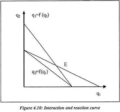
Since b, b₁ and b₂ are all positive. A rise of either duopoly’s output will cause a reduction of the other’s optimism output. The reaction functions are linear and it is as shown in the following diagram. Equilibrium is shown by the interaction of point for reaction curves at point ‘e’.

 

The Cournot Nash equilibrium equation is at E. The strategies are consists of quantity. In the Cournot game, the Nash equilibrium has the property of stability.

Criticism:

The Cournot model is criticized on various points. Firm A believes that if it changes q1 another firm will not respond by changing q. The strategies are decided in terms of prices rather than quantities. The Nash equilibrium is much different. The Cournot model assumes that firms pick quantities rather than prices. That means an auctioneer chooses the price to equate supply and demand.

Cournot Duopoly Model: Continuous Strategies:

The earliest duopoly model was developed in 1938. It is developed by the French economist Augstin Cournot. He has noted that this game has a unique equilibrium when demand curves are linear. The Cournot game has a continuous strategy space even without mixing. If a game has a continuous strategy set then it is not always easy to depict the strategic form and outcome matrix is an extensive form as a tree. In order to present Cournot game, new notation will be useful.

i. The Cournot game model is a duopoly in which two firms chooses output levels in competition with each other.

ii. There are the two players. The firms are Apex and Brydox.

iii. Apex and Brydox simultaneously choose quantities qa and qb from the set (0, ∞)

iv. Production cost is zero.

Demand is a function of the total quantity sold in the market.

Suppose the game is co-operative then firms would end up producing somewhere on the 45° line in figure. Total output is the monopoly output and it maximizes the sum of payoffs. More specifically, the monopoly output maximizes PQ = (120-Q) Q with respect to the total output of Q. It is resulting in first order condition as 120-2q = 0. It implies a total output of 60 and a price of 60. In order to decide how much of that output of 60 should be produced by each firm. The firm’s output should be located on the 45° line. Such output would be a zero sum co-operative game. It is an example of bargaining between firms.

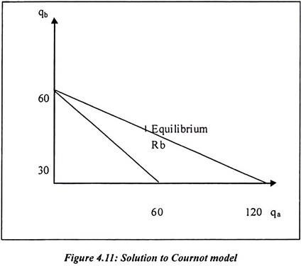
But since the Cournot game is non-co-operative game. The strategy combinations such that qa + qb = 60. It is not necessarily equilibrium despite their Pareto optimality. Each firm produces about quantity he wants to produce and unaware about rivals plan of production. In order to find Nash equilibrium in Cournot game, we need a reaction function. If Brydox produces output then Apex would produce the monopoly output of 60.

If Brydox produced qb = 120 or greater, the market price would fall to zero and Apex would choose to produce zero. The best response function is found by maximizing Apex’s payoff. It is given in following equation with respect to his strategy qa.

This generates the first order condition as follows:

or

The reaction function of the two firms is labeled as Ra and Rb in figure. They cross point c which is the Cournot-Nash-Equilibrium. It is also the Nash equilibrium when the strategies consist of quantities. Algebraically, if it is solved then the two reaction functions for qa and qb, which generates unique equation (qa = 40, qb = 40).The equilibrium price is also 40, co-incidentally. In the Cournot game, the Nash equilibrium has the particularly property of stability.

If we assume that the initial strategy combination is point x in figure, then it moves the profile closer to equilibrium. But this is special to the Cournot game and Nash equilibrium is not always stable in this way.

Critics of Model:

Above model is criticized on the following points:

1. In Nash equilibrium, Apex believes that if he changes qa Brydox will not respond by changing qb.

2. Another objection is that the strategy set are specified to be quantities.

3. If strategies are prices rather than quantities the Nash equilibrium is much different.

4. What happens when one firm’s costs are positive and information is incomplete?

Solution to Cournot Model by Stackelberg Equilibrium:

Stackelberg equilibrium differs from Cournot equilibrium. In Stackelberg equilibrium, one firm gets to choose its quantity first who are Stackelberg leader and the other players is Stackelberg follower. The distinguishing characteristic of Stackelberg equilibrium is that one player gets to commit him first. In the following figure, Apex moves first inter temporally. Suppose moves were simultaneous but Apex could commit himself to a certain strategy. The same equilibrium would be reached as long as Brydox was not able to commit himself.

Algebraically, since Apex forecasts Brydox’s output to be:

Apex can substitute this into his payoff function in (34) and obtaining:

If the above function maximizing with respect to q_a then it yields the first order condition:

Which generates qa = 60. Once Apex chooses this output, Brydox chooses his output which is to be qb = 30.The market price is 30 for both firms. Apex has benefited from his status as Stackelberg leader.