3 Static Properties of a General Equilibrium State

Three static properties are observed in a general equilibrium solution, reached with a free competitive market mechanism:

(a) Efficient allocation of resources among firms (equilibrium of production).

(b) Efficient distribution of the commodities produced between the two consumers (equilibrium of consumption).

(c) Efficient combination of products (simultaneous equilibrium of production and consumption).

These properties are called marginal conditions of Pareto optimality or Pareto efficiency. A situation is defined as Pareto optimal (or efficient) if it is impossible to make anyone better-off without making someone worse-off. In the following paragraphs we discuss briefly the three optimality properties that are observed in a general equilib­rium state.

(a) Equilibrium of production (efficiency in factor substitution):

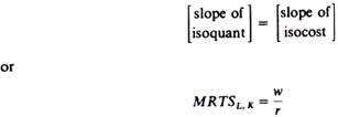
Equilibrium of production requires the determination of the efficient distribution of the available productive factors among the existing firms (efficiency in factor substitution). We know that the firm is in equilibrium if it chooses the factor combination (for producing the most lucrative level of output) which minimizes its cost. Thus the equilibrium of the firm requires that

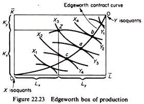
where w and r are the factor prices prevailing in the market and MRTS is the marginal rate of technical substitution between the factors. The joint equilibrium of production of the two firms in our simple model can be derived by the use of the Edge-worth box of production. On the axes of this construct we measure the given quantities of the factors of production, K and L (figure 22.23). The isoquants of commodity X are plotted with origin the south-west corner and the isoquants of y are plotted with origin the north-east corner.

The locus of points of tangency of the X and Y isoquants is called the Edge-worth contract curve of production. This curve is of particular importance because it includes the efficient allocations of K and L between the firms.

Each point of the Edge-worth box shows a specific allocation of K and L in the production of commodities X and y. Such an allocation defines six variables the amounts of Y and X produced and the amounts of capital and labour allocated to the production of Y and X.

For example point Z shows that:

X₃ is the quantity produced of commodity X

Y₂ is the quantity produced of commodity Y

K_x is the amount of capital allocated to the production of X₃

K_y is the amount of capital allocated to the production of Y₂

L_x is the amount of labour allocated to the production of X₃

L_y is the amount of labour allocated to the production of Y₂

However, not all points of the Edge-worth box represent efficient allocations of the available resources. Given that K and L are limited in supply, their use should produce the greatest possible output. An allocation of inputs is efficient if the produced combination of X and Y is such that it is impossible to increase the production of one commodity without decreasing the quantity of the other.

From figure 22.23 we see that efficient production takes place on the Edge-worth contract curve. It is impossible to move to a point off this curve without reducing the quantity of at least one commodity. Point Z is a point of inefficient production, since a reallocation of K and L between the two commodities (or firms) such as to reach any point from a to b leads to a greater production of one or both commodities.

Since the Edge-worth contract curve of production is the locus of tangencies of the X and Y isoquants, at each one of its points the slopes of the isoquants are equal:

In our simple general equilibrium model the firms, being profit maximisers in competitive markets, will be in equilibrium only if they produce somewhere on the Edgeworth contract curve. This follows from the fact that the factor prices facing the producers are the same, and their profit maximisation requires that each firm equates its MRTS_{L k} with the ratio of factor prices w/r

MRTS^x_L,_k = MRTS^y_L,_k = w/r (1)

In summary. The general equilibrium of production occurs at a point where the MRTS_L,_k is the same for all the firms, that is, at a point which satisfies the Pareto- optimality criterion of efficiency in factor substitution the general equilibrium of production is a Pareto-efficient allocation of resources. The production equilibrium is not unique, since it may occur at any point along the Edgeworth contract curve there is an infinite number of possible Pareto-optimal production equilibria.

However, with perfect competition, one of these equilibria will be realized, the one at which the (‘equalised’ between the firms) MRTS_L,_K is equal to the ratio of the market factor prices w/r. That is, with perfect competition general equilibrium of production occurs where condition (1) is satisfied.

If the factor prices are given, from the Edgeworth box of production we can determine the amounts of X and Y which maximise the profits of firms. However, in a general equilibrium, these quantities must be equal to those which consumers want to buy in order to maximise their utility. Consumers decide their purchases on the basis of the prices of commodities, P_x and P_y.

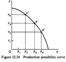
Thus, in order to bring together the production side of the system with the demand side, we must define the equilibrium of the firms in the product space, using as a tool the production possibility curve of the economy. This is derived from the Edgeworth contract curve of production, by mapping its points on a graph on whose axes we measure the quantities of the final commodities X and Y.

From each point of the Edgeworth contract curve of produc­tion we can read off the maximum obtainable quantity of one commodity, given the quantity of the other. For example, point a in figure 22.23 shows that, given the quantity of X is X₃, the maximum quantity of Y that can be produced (with the given factors K and L) is Y₃.

The X₃, Y₃ combination is presented by point a’ in figure 22.24. Similarly, point b of the Edge-worth contract curve of production shows that, given X₄, the maximum amount of Y that the economy can produce is Y₂. Point b’ in figure 22.24 is the mapping of b from the factor space to the production space.

In summary, the production possibility curve of an economy is the locus of all Pareto-efficient outputs, given the resource endownment (K and L) and the state of technology. This curve shows the maximum quantity of a good obtainable, given the quantity of the other good. At any point on the curve all factors are optimally (efficiently) employed. Any point inside the curve is technically inefficient, implying unemployed resources. Any point above the curve is unattainable, unless additional resources or a new technology or both are found.

The production possibility curve is also called the product transformation curve because it shows how a commodity is ‘transformed’ into another, by transferring some factors from the production of one commodity to the other.

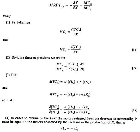
The negative of the slope of the production possibility curve is called the marginal rate of (product) transformation, MRPT_xy and it shows the amount of Y that must be sacrificed in order to obtain an additional unit of X. The economic meaning of the transformation curve is the rate at which a commodity can be transformed into another. By definition

MRPT_x,_y = dY/dX

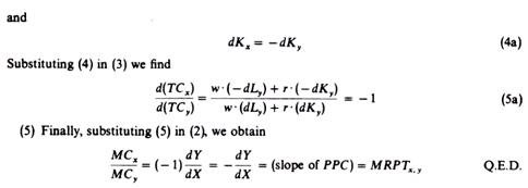
Since dY/dX is negative, the MRPT is a positive number. It can be shown that the MRPT_xy is equal to the ratio of the marginal costs of the two products

In perfect competition the profit-maximising producer equates the price of the commodity produced to the long-run marginal cost of production

MC_X = P_x and

MC_y = P_y

Therefore the slope of the production possibility curve is also equal to the ratio of the prices at which X and Y will be supplied by perfectly competitive industries

MRPT_x,y = MC_x / MC_y = P_x / P_y …(2)

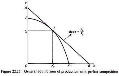
Given the commodity prices, general equilibrium of production is reached at the point on the production transformation curve that has a slope equal to the ratio of these prices. Such a general equilibrium of production is shown in figure 22.25. Assume that the market prices of commodities define the slope of the line AB. The ratio 0A/0B measures the ratio of the marginal cost of and hence the supply price of X to that of y.

The general equilibrium product-mix from the point of view of firms is given by point T. The two firms are in equilibrium producing the levels of output Y_e and X_e.

(b) Equilibrium of consumption (efficiency in distribution of commodities):

We must now show how each consumer, faced with the market prices P_x and P_y, reaches equilibrium, that is, maximises his satisfaction. From the theory of consumer behaviour we know that the consumer maximises his utility by equating the marginal rate of substitution of the two commodities (slope of his indifference curves) to the price ratio of the commodities. Thus the condition for consumer equilibrium is

MRS_x,_y = P_x /P_y

Since both consumers in perfectly competitive markets are faced with the same prices the condition for joint or general equilibrium of both consumers is

MRS^A_x,_y = MRS^B_x,_y = P_x /P_y (3)

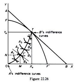
This general equilibrium of consumption for the product mix Y^e, X^e is shown in figure 22.26. We construct an Edgeworth box for consumption with the precise dimensions Y^e and X^e by dropping from point T (on the product transformation curve) lines parallel to the commodity axes. We next plot the indifference curves of consumer A with origin the south-west corner, and the indifference curves of B with origin the north-east corner.

Any point in the Edgeworth consumption box shows six variables: the total quanti­ties Y^e and X^e, and a particular distribution of these quantities between the two consumers. However, not all distributions are efficient in the Pareto sense.

A Pareto- efficient distribution of commodities is one such that it is impossible to increase the utility of one consumer without reducing the utility of the other. From figure 22.26 it is seen that only points of tangency of the indifference curves of the two consumers represent Pareto-efficient distributions. The locus of these points is called the Edge- worth contract curve of consumption. It should be clear that at each point of this curve the following equilibrium condition is satisfied

MRS^A_x,_y = MRS^B_x,_y

Thus for a given product-mix (such as T, which we are considering) there is an infinite number of possible Pareto-optimal equilibria of distribution: the equilibrium of consumption is not unique, since it can occur at any point of the contract curve of consumption. However, with perfect competition, only one of these points is consist­ent with the general equilibrium of the system. This is the point of the contract curve where the (‘equalised’) MRS_x,_y of the consumers is equal to the price ratio of the commodities, that is, where condition (3) is fulfilled.

In figure 22.26 the equilibrium of the consumers is defined by point T. Consumer A reaches the utility level implied by the indifference curve A₂, buying 0M of X and ON of Y. Consumer B reaches the utility level implied by the indifference curve B₄, buying the remaining quantities MX_e of X and NY_e of Y.

(c) Simultaneous equilibrium of production and consumption (efficiency in product-mix):

From the discussion of the preceding two sections it follows that the general equilibrium of the system as a whole requires the fulfillment of a third condition, namely that the marginal rate of product transformation (slope of the PPC) be equal to the marginal rate of substitution of the two commodities between the consumers

MRPT_x,y = MRS^A_x,_y = MRS^B_x,_y

In perfect competition this condition is satisfied, since, from expression (2)

MRPT_x,_y = P_x/P_y

and from expression (3)

MRS^A_x,_y = MRS^B_x,_y = P_x/P_y

so that

MRPT_{X, y} = MRS^A_x,_y = MRS^B_x,_y (4)

This is the third condition of Pareto efficiency. It refers to the efficiency of product substitution (or optimal composition of output). Since the MRPT shows the rate at which a good can be transformed into another in production, and the MRS shows the rate at which the consumers are willing to exchange one good for another, the system is not in equilibrium unless the two ratios are equal. Only then the production sectors’ plans are consistent with the household sectors’ plans, and the two are in equilibrium.

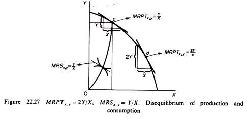
A simple numerical example may illustrate the argument. Suppose that the MRPT_X,y is 2 Y/X, while the MRS_X,y — Y/X. The economy can produce two units of Y by sacrificing one unit of X, while the consumers are willing to exchange one unit of X for one unit of Y. In figure 22.27 the inequality of the two ratios is shown by points c and d.

Apparently firms produce a smaller quantity of Y and a larger quantity of X relative to the preferences of the consumers. Given the assumption of consumer sovereignty, firms must reduce X and increase the production of Y for the attainment of general equilibrium. The economic meaning of the third efficiency criterion is that the combination of outputs must be optimal from both the consumers’ and the producers’ point of view.

In summary, with perfect competition (and no discontinuities and with constant returns to scale) the simple two-factor, two-commodity, two-consumer system has a general equilibrium solution, in which three Pareto-efficiency conditions are satisfied:

1. The MRS between the two goods is equal for both consumers. This efficiency in distribution implies optimal allocation of the goods among consumers.

2. The MRTS between the two factors is equal for all firms. This efficiency in factor substitution implies optimal allocation of the factors among the two firms.

3. The MRS and the MRPT are equal for the two goods. This efficiency in product- mix implies optimal composition of output in the economy and thus optimal alloca­tion of resources.

Whether such a general equilibrium solution (on the PPC) is desirable for the society as a whole is another question, which is the core of Welfare Economics.