The following article will guide you about how are factor prices determined under imperfect competition.
The Marginal productivity theory of Distribution, as explained by J. B. Clark and others, is applicable to the determination of factor prices under perfect competition. But Mrs. Robinson has extended its application to all types of market situations. So, the theory, as modified by them can be applied to determine factor price under imperfect competition and monopoly.
The modified theory can be explained as follows:
In the original theory it was stated that the price of a factor and its earnings would be equal to the value of its marginal physical product (MPP of a factor multiplied by the price of the product of the firm. But the modified theory states that the relevant concept for the factor price determination is the marginal revenue product (MPP x MR) of a factor, not the value of its marginal product (VMP). Under perfect competition AR is always equal to MR and thus, VMP of a factor is equal to its MRP. But under imperfect competition and monopoly MRP of factor is less than its VMP because MR<P.
ADVERTISEMENTS:
The modified theory states that in equilibrium the marginal revenue product of a factor, say, labour, under imperfect competition and monopoly becomes equal to its marginal wage (not to average wage). In other words the MRP of a variable factor, say, labour, becomes equal to marginal wage (not to average wage). When the competition is perfect, average wage of labour (AW) becomes equal to marginal wage (MW) and AW curve becomes identical with MW curve OA as a result MRP of labour = MW = AW.
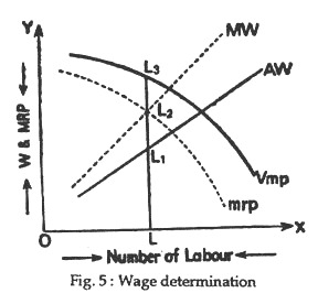
But, in the case of imperfect competition and monopoly as average wage increases with the increase in the employment of labour MW>AW, i.e., the MW curve lies above the AW curve. So, an employer would employ a factor up to that point where it’s MRP=MW. But, all the units of a factor (say, labour) are to be paid wages at the same rate (i.e., AW), the equilibrium or market determined wage becomes less than both VMP and MRP of labour. This point can be seen in Fig.5.
In Fig. 5 the VMP curve and MRP curve are the value of marginal product and the marginal revenue product curve, respectively under imperfect competition or monopoly. As MR<P or AR the MRP curve lies below the VMP curve. Thus, MW curve is the marginal wage curve and AW is the average wage curve. In such a situation, as average wage increases with the increase in employment, MW curve lies above the AW curve.
ADVERTISEMENTS:
In Fig. 5 an employer would employ OL number of labour because here MRP of labour = M W (at L2). But here the rate of wage, i.e., average wage becomes LL1 and wage rate is less than both marginal revenue product (LL2) and value of marginal product (LL3) of labour. So here the wage-rule is not equal to the VMP of labour as is observed in perfect competition. In this case the wage rate is lower by L2L3 and this represents the exploitation of an average worker.
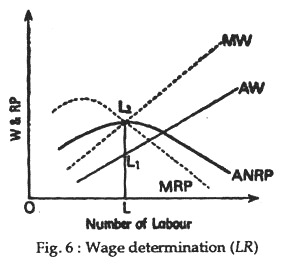
In the long run, an employer would continue to employ labour until as under perfect competition, marginal wage, marginal revenue product and average revenue product (ARP) all become equal. This point is illustrated can in Figure 6.
Fig. 6 shows that, when OL numbers of labour are employed, marginal wages i.e., LL2 = MRP, i.e., LL2 and ARP which is also LL2. Here the rate of wage or AW becomes LL1.
So, the theory of wage determination under non-pure competition is different from wage determination under pure competition. The entry of trade unions into the labour market makes our analysis. The same thing happens when the government passes minimum wage rate. Similarly, import of goods at a cheap price may reduce wages.

